
the Creative Commons Attribution 4.0 License.
the Creative Commons Attribution 4.0 License.
 | 20 Nov 2025
Spectral Analysis of Groundwater Level Time Series for Robust Estimation of Aquifer Response Times
Abstract. Groundwater resources represent Germany's most important source of freshwater but they are increasingly under pressure. Climate change, societal developments, and rising abstraction rates are impacting subsurface storage in ways that are currently difficult to predict, affecting both the quantity and quality of groundwater. To ensure sustainable groundwater management, it is crucial to evaluate the intrinsic and spatially variable vulnerability of groundwater systems, especially to prepare for the effects of hydrological extremes. In this context, the groundwater response time, defined as the timescale over which a groundwater system responds or adjusts to changes in external or internal conditions, serves as a valuable indicator for vulnerability assessments. Unlike traditional methods, we propose estimating response times through spectral analysis of groundwater level data. Time series from nearly 200 selected observation wells across Bavaria in Southern Germany were processed and transformed into the spectral domain. Corresponding recharge time series were extracted from high-resolution hydrological model outputs. By integrating these data with hydrogeomorphic information, we fitted a semi-analytical model to the groundwater level spectra to obtain aquifer response times. The semi-analytical solution for the spectral domain accurately reproduced the majority of observed groundwater level spectra. Most estimated response times fall between roughly 50 and 300 days. Significant correlation were found between the response time and the depth of the groundwater table. Groundwater systems exhibiting longer response times are interpreted as more resilient to drought conditions and therefore potentially better suited for groundwater abstraction than aquifers with shorter response times.
-
Notice on discussion status
The requested preprint has a corresponding peer-reviewed final revised paper. You are encouraged to refer to the final revised version.
-
Preprint
(22514 KB)
-
The requested preprint has a corresponding peer-reviewed final revised paper. You are encouraged to refer to the final revised version.
- Preprint
(22514 KB) - Metadata XML
- BibTeX
- EndNote
- Final revised paper


Journal article(s) based on this preprint
Groundwater is vital but increasingly stressed by climate change and rising water demand. This study estimates how quickly aquifers respond to changes in recharge using a signal-analysis method. Most aquifers reacted within one to ten months, while deeper responded more slowly and proved more resilient to short droughts. The method uses existing monitoring data, offering a practical way to identify vulnerable aquifers and guide groundwater management under climate change.
Interactive discussion
Status: closed
-
RC1: 'Comment on egusphere-2025-5666', Anonymous Referee #1, 27 Dec 2025
- AC1: 'Reply on RC1', Timo Houben, 13 Apr 2026
-
RC2: 'Comment on egusphere-2025-5666', Gunnar Lischeid, 09 Feb 2026
Assessing the vulnerability of groundwater systems is one of the key challenges of groundwater research, not the least due to presumed increasing probability of extreme events. Most of the work done so far is based on modelling studies. Houben et al. followed a different approach based on earlier work by Zhang and Schilling. I agree that spectrum analysis has great and still massively underrated potential in this regard. It is to the credit of this work that it draws the attention of the scientific community to this. However, the devil is in the details.
- My major criticism is, that this study completely ignores the major source of low-pass filtering. The approach by Liang and Zhang (2013) works under the ideal conditions of tailored numeric experiments. Even then the effects on power spectra are fairly small and are restricted to small distances from the constant head boundary. In real world settings, though, these effects are hardly discernible due to the much stronger impact of vadose zone low-pass filtering. In contrast to the effect described by Liang and Zhang, however, the latter starts to manifest in the high frequency part. This phenomenon is closely related to the second law of thermodynamics (dissipation is the strongest for the high energy part of the spectrum). It applies likewise to soil temperature, electromagnetic waves, etc. Consequently, it doesn’t come as a surprise that the spectra are consistently underestimated for shallow groundwater sites and overestimated for deep groundwater sites (Fig. 7).
- 58-62: What is perceived here as an interference signal is actually the main driver of the low-pass filtering effect: It is the vadose zone rather than the aquifer – have a look at Fig. 4, 5, and 6 in Tsypin et al. (2025, https://doi.org/10.1016/j.jhydrol.2025.133193) or at Liesch and Wunsch (2019, https://doi.org/10.1016/j.jhydrol.2019.02.060). The thicker the vadose zone, the more pronounced is the low-pass filtering effect. The pore space in the aquifer is fully saturated, and water is hardly compressible. Thus, how could the aquifer buffer any input (except by discharging to the constant head boundary)?
- 98-100, 220-223: Cut-off frequencies, that is, the change of slope is a nice index to compare different time series. But it comes with two major problems: Firstly, deep groundwater head dynamics usually exhibits pronounced persistency with Hurst coefficients exceeding 0.5. Thus, legacy effects will last for very long (Koutsoyiannis 2013, http://dx.doi.org/10.1080/02626667.2013.804626). Actually, there is no upper limit of response time at all for very fundamental reasons. Secondly, such clear breaks of slope are limited to time series with rather low degrees of low-pass filtering like stream discharge. In contrast, power spectra of deep groundwater head time series often do not show any clear cut-off frequencies. See, e.g., observed groundwater head spectra (Fig. 4) in Zhang and Schilling (2004, https://doi.org/10.1029/2003WR002094) or Fig. 4 in Tsypin et al. (2025, https://doi.org/10.1016/j.jhydrol.2025.133193). There is no physical reason why low-pass filtering should stop at a certain frequency. It is just a matter of the intensity of the low-pass filtering process. Please comment.
- 152-156: Removing linear trends distorts the power spectrum. Trends do not develop independent from the spectral signatures but are an inevitable consequence of the low-pass filtering process which results in increasingly more smooth time series. Consequently, the length of periods of monotonic rise or fall increases and thus the probability to identify significant trends (Koutsoyiannis 2006, https://doi.org/10.1016/j.jhydrol.2005.02.030; Lischeid et al. 2021, https://doi.org/10.1016/j.jhydrol.2021.126096). This holds even for random white noise time series.
- 273-276: It is indicative that the paper does neither report on transmissivity nor on storage values. Other than the authors I would ascribe these uncertainties to disregarding the vadose zone effect on low-pass filtering (see above) rather than to uncertainties of flow line length determination. Please comment.
- 12-15, 300-306: The statement “Groundwater systems exhibiting longer response times are interpreted as more resilient to drought conditions and therefore potentially better suited for groundwater abstraction than aquifers with shorter response times” holds only in the short-term when the response time is long compared to the timescale of dry spells. But long-term buffering comes with the price of very slow and delayed recovery. Increasingly longer dry spells and extended periods of a monotonic decrease of groundwater head and total water storage which are now abundant in Central Europe (Xanke and Liesch 2022, https://doi.org/10.1007/s10040-021-02448-3; Wunsch et al. 2022, https://doi.org/10.1038/s41467-022-28770-2) question such recommendations. Please comment.
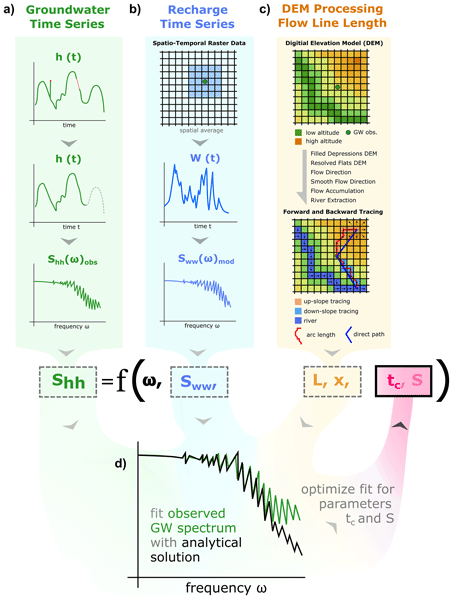
- Figure 1: Please explain the b) and c) panels. It is a little bit unusual and confusing to have two panels b) and c) each.
- Figure 2: Correct “lenth” in the figure caption.
- A3: I guess the term “spectral analysis” refers to the whole procedure rather than to the power spectra of groundwater head time series in particular, is that right? Otherwise, frequencies should always be < 1. Please clarify.
- A8: This spectrum seems to be indicative for a confined aquifer where short-term fluctuations are induced by atmospheric pressure variation, resulting in a remarkable atypical large share of variance in the high-frequency range.
Citation: https://doi.org/10.5194/egusphere-2025-5666-RC2 - AC2: 'Reply on RC2', Timo Houben, 13 Apr 2026
Peer review completion


Interactive discussion
Status: closed
-
RC1: 'Comment on egusphere-2025-5666', Anonymous Referee #1, 27 Dec 2025
Summary
The manuscript by Houben et al presents a methodology that combines time series analysis, GIS and analytical modelling to estimate the average response time of aquifers in a large, regional data set of groundwater level time series from observation wells in the upper Danube river basin. The approach rests on existing findings by (i.a. Houben et al., 2022; Liang & Zhang; Zhang & Schilling, 2004) regarding temporal scaling of groundwater head and relation to aquifer geometry, properties and recharge. Here, the focus was on estimating at each location the characteristic time scale, a single value that quantifies the rate at which an aquifer responds to an external stress. This value is then briefly framed as a characteristic to quantify aquifer vulnerability to drought and criteria for selection of aquifers for abstraction. While the approach generally is sound, my primary concern with this paper is that the value of the analysis is not apparent when compared to other studies that require fewer data, assumptions, and less effort, such as the referenced study by Kumar et al. (2016) or Ebeling et al. (2025). What benefit does the characteristic time scale provide versus the current standard method in groundwater drought analysis using correlation times of SP(E)I vs SGI for example or e.g. cross-correlations (e.g., Bloomfield & Marchant, 2013; Ebeling et al., 2025)? I think the authors need to reflect on - and clarify this before the manuscript can be considered for publication. Below find specific comments:
- The recharge data that is used needs more description for readers not familiar with mHM. What does it represent within the model context, is it the input to a groundwater component?
- Is the recharge calibrated on observation data (lysimeter) or is it the residual from runoff and soil moisture? This distinction is important for understanding the reliability of the input data.
- Given the difficulty of estimating recharge on short temporal scales my expectation would be that this is a significant uncertainty for the study. Discuss the challenges and uncertainties associated with estimating recharge at short temporal scales, and how these uncertainties may affect the study's conclusions.
- Also related to recharge, in L150 you state that the recharge is extracted from multiple cells and spatially averaged. Why and how?
- This also assumes localized recharge for all wells, which is a standard approach in 1D modelling approaches. You are however using a 2D conceptualization, where the standard perceptual models consider recharge/intermediate/discharge zones (e.g. Tóthian basins or Winter’s hydrologic landscapes) Clarify the assumption that localized recharge is appropriate for all wells. Discuss how this assumption fits and acknowledge any additional uncertainties introduced.
- Improve the description of the groundwater level data set that was used. Currently it is not clear what temporal resolution the data has, or if it is regular.
- The outlier handling using the inter-quartile range is generally inappropriate for groundwater level time series due to their seasonality and thus potential for outliers that are not overall extreme values. Likely this is not important when the time series are transformed into the frequency domain. However, please elaborate on this issue.
- The entire section LL183-193 is hard to follow and should be rewritten. Specific questions in this sections are:
- L183: What is meant by tracing “back” the path of the water particle towards the river?
- The sentence L189-190 is hard to understand. Is this the flow path from water divide to river?
- L191 Why was the direct distance applied?
- In LL242ff does this analysis only pertain to all time series or only good fits?
- In L290 you refer to intermediate frequencies as the “onset of filtering related to the groundwater response time”. This description does not help with intuition. Can you clarify what this might mean process-wise?
- Finally, (Ebeling et al., 2025; Kumar et al., 2016) carried out studies in the same regions and also link deeper wells to longer response times, although here responses of multiple years are identified. Reflect on the differences between tc and accumulation times, and how tc can be understood and used for groundwater drought analysis compared to current practice.
Technical comments
- In abstract you write “nearly 200 … wells”, but in section 2.2.2 it is 224.
- L46ff: Clarify how variability in recession constants are related to the difficulty in defining drought extent? I challenge that defining drought extent is really that difficult, it is a factor of the systems hydraulic memory (Changnon, 1987).
- Fig1 Please elaborate on b,c in caption
- Fig 2 Please elaborate on a,b,c,d in the caption. Also the arc length and direct path are not clearly visable. Please improve. For a and b write descriptive titles for each step.
- L187 noise --> noisy
References
Bloomfield, J. P., & Marchant, B. P. (2013). Analysis of groundwater drought building on the standardised precipitation index approach. Hydrol. Earth Syst. Sci., 17(12), 4769-4787. https://doi.org/10.5194/hess-17-4769-2013
Changnon, S. A. (1987). Detecting drought conditions in Illinois. Circular no. 169.
Ebeling, P., Musolff, A., Kumar, R., Hartmann, A., & Fleckenstein, J. H. (2025). Groundwater head responses to droughts across Germany. Hydrol. Earth Syst. Sci., 29(13), 2925-2950. https://doi.org/10.5194/hess-29-2925-2025
Houben, T., Pujades, E., Kalbacher, T., Dietrich, P., & Attinger, S. (2022). From Dynamic Groundwater Level Measurements to Regional Aquifer Parameters— Assessing the Power of Spectral Analysis. Water Resources Research, 58(5). https://doi.org/10.1029/2021wr031289
Kumar, R., Musuuza, J. L., Van Loon, A. F., Teuling, A. J., Barthel, R., Ten Broek, J., Mai, J., Samaniego, L., & Attinger, S. (2016). Multiscale evaluation of the Standardized Precipitation Index as a groundwater drought indicator. Hydrol. Earth Syst. Sci., 20(3), 1117-1131. https://doi.org/10.5194/hess-20-1117-2016
Liang, X., & Zhang, Y.-K. (2013). Temporal and spatial variation and scaling of groundwater levels in a bounded unconfined aquifer. Journal of Hydrology, 479, 139-145. https://doi.org/10.1016/j.jhydrol.2012.11.044
Zhang, Y. K., & Schilling, K. (2004). Temporal scaling of hydraulic head and river base flow and its implication for groundwater recharge. Water Resources Research, 40(3), W035041-W035049.
Citation: https://doi.org/10.5194/egusphere-2025-5666-RC1 - AC1: 'Reply on RC1', Timo Houben, 13 Apr 2026
-
RC2: 'Comment on egusphere-2025-5666', Gunnar Lischeid, 09 Feb 2026
Assessing the vulnerability of groundwater systems is one of the key challenges of groundwater research, not the least due to presumed increasing probability of extreme events. Most of the work done so far is based on modelling studies. Houben et al. followed a different approach based on earlier work by Zhang and Schilling. I agree that spectrum analysis has great and still massively underrated potential in this regard. It is to the credit of this work that it draws the attention of the scientific community to this. However, the devil is in the details.
- My major criticism is, that this study completely ignores the major source of low-pass filtering. The approach by Liang and Zhang (2013) works under the ideal conditions of tailored numeric experiments. Even then the effects on power spectra are fairly small and are restricted to small distances from the constant head boundary. In real world settings, though, these effects are hardly discernible due to the much stronger impact of vadose zone low-pass filtering. In contrast to the effect described by Liang and Zhang, however, the latter starts to manifest in the high frequency part. This phenomenon is closely related to the second law of thermodynamics (dissipation is the strongest for the high energy part of the spectrum). It applies likewise to soil temperature, electromagnetic waves, etc. Consequently, it doesn’t come as a surprise that the spectra are consistently underestimated for shallow groundwater sites and overestimated for deep groundwater sites (Fig. 7).
- 58-62: What is perceived here as an interference signal is actually the main driver of the low-pass filtering effect: It is the vadose zone rather than the aquifer – have a look at Fig. 4, 5, and 6 in Tsypin et al. (2025, https://doi.org/10.1016/j.jhydrol.2025.133193) or at Liesch and Wunsch (2019, https://doi.org/10.1016/j.jhydrol.2019.02.060). The thicker the vadose zone, the more pronounced is the low-pass filtering effect. The pore space in the aquifer is fully saturated, and water is hardly compressible. Thus, how could the aquifer buffer any input (except by discharging to the constant head boundary)?
- 98-100, 220-223: Cut-off frequencies, that is, the change of slope is a nice index to compare different time series. But it comes with two major problems: Firstly, deep groundwater head dynamics usually exhibits pronounced persistency with Hurst coefficients exceeding 0.5. Thus, legacy effects will last for very long (Koutsoyiannis 2013, http://dx.doi.org/10.1080/02626667.2013.804626). Actually, there is no upper limit of response time at all for very fundamental reasons. Secondly, such clear breaks of slope are limited to time series with rather low degrees of low-pass filtering like stream discharge. In contrast, power spectra of deep groundwater head time series often do not show any clear cut-off frequencies. See, e.g., observed groundwater head spectra (Fig. 4) in Zhang and Schilling (2004, https://doi.org/10.1029/2003WR002094) or Fig. 4 in Tsypin et al. (2025, https://doi.org/10.1016/j.jhydrol.2025.133193). There is no physical reason why low-pass filtering should stop at a certain frequency. It is just a matter of the intensity of the low-pass filtering process. Please comment.
- 152-156: Removing linear trends distorts the power spectrum. Trends do not develop independent from the spectral signatures but are an inevitable consequence of the low-pass filtering process which results in increasingly more smooth time series. Consequently, the length of periods of monotonic rise or fall increases and thus the probability to identify significant trends (Koutsoyiannis 2006, https://doi.org/10.1016/j.jhydrol.2005.02.030; Lischeid et al. 2021, https://doi.org/10.1016/j.jhydrol.2021.126096). This holds even for random white noise time series.
- 273-276: It is indicative that the paper does neither report on transmissivity nor on storage values. Other than the authors I would ascribe these uncertainties to disregarding the vadose zone effect on low-pass filtering (see above) rather than to uncertainties of flow line length determination. Please comment.
- 12-15, 300-306: The statement “Groundwater systems exhibiting longer response times are interpreted as more resilient to drought conditions and therefore potentially better suited for groundwater abstraction than aquifers with shorter response times” holds only in the short-term when the response time is long compared to the timescale of dry spells. But long-term buffering comes with the price of very slow and delayed recovery. Increasingly longer dry spells and extended periods of a monotonic decrease of groundwater head and total water storage which are now abundant in Central Europe (Xanke and Liesch 2022, https://doi.org/10.1007/s10040-021-02448-3; Wunsch et al. 2022, https://doi.org/10.1038/s41467-022-28770-2) question such recommendations. Please comment.
- Figure 1: Please explain the b) and c) panels. It is a little bit unusual and confusing to have two panels b) and c) each.
- Figure 2: Correct “lenth” in the figure caption.
- A3: I guess the term “spectral analysis” refers to the whole procedure rather than to the power spectra of groundwater head time series in particular, is that right? Otherwise, frequencies should always be < 1. Please clarify.
- A8: This spectrum seems to be indicative for a confined aquifer where short-term fluctuations are induced by atmospheric pressure variation, resulting in a remarkable atypical large share of variance in the high-frequency range.
Citation: https://doi.org/10.5194/egusphere-2025-5666-RC2 - AC2: 'Reply on RC2', Timo Houben, 13 Apr 2026
Peer review completion
Journal article(s) based on this preprint
Groundwater is vital but increasingly stressed by climate change and rising water demand. This study estimates how quickly aquifers respond to changes in recharge using a signal-analysis method. Most aquifers reacted within one to ten months, while deeper responded more slowly and proved more resilient to short droughts. The method uses existing monitoring data, offering a practical way to identify vulnerable aquifers and guide groundwater management under climate change.
Viewed
| HTML | XML | Total | BibTeX | EndNote | |
|---|---|---|---|---|---|
| 2,116 | 2,361 | 167 | 4,644 | 169 | 136 |
- HTML: 2,116
- PDF: 2,361
- XML: 167
- Total: 4,644
- BibTeX: 169
- EndNote: 136
Viewed (geographical distribution)
| Country | # | Views | % |
|---|
| Total: | 0 |
| HTML: | 0 |
| PDF: | 0 |
| XML: | 0 |
- 1

Christian Siebert
Thomas Kalbacher
Mariaines Di Dato
Thomas Fischer
Sabine Attinger
The requested preprint has a corresponding peer-reviewed final revised paper. You are encouraged to refer to the final revised version.
- Preprint
(22514 KB) - Metadata XML
Summary
The manuscript by Houben et al presents a methodology that combines time series analysis, GIS and analytical modelling to estimate the average response time of aquifers in a large, regional data set of groundwater level time series from observation wells in the upper Danube river basin. The approach rests on existing findings by (i.a. Houben et al., 2022; Liang & Zhang; Zhang & Schilling, 2004) regarding temporal scaling of groundwater head and relation to aquifer geometry, properties and recharge. Here, the focus was on estimating at each location the characteristic time scale, a single value that quantifies the rate at which an aquifer responds to an external stress. This value is then briefly framed as a characteristic to quantify aquifer vulnerability to drought and criteria for selection of aquifers for abstraction. While the approach generally is sound, my primary concern with this paper is that the value of the analysis is not apparent when compared to other studies that require fewer data, assumptions, and less effort, such as the referenced study by Kumar et al. (2016) or Ebeling et al. (2025). What benefit does the characteristic time scale provide versus the current standard method in groundwater drought analysis using correlation times of SP(E)I vs SGI for example or e.g. cross-correlations (e.g., Bloomfield & Marchant, 2013; Ebeling et al., 2025)? I think the authors need to reflect on - and clarify this before the manuscript can be considered for publication. Below find specific comments:
Technical comments
References
Bloomfield, J. P., & Marchant, B. P. (2013). Analysis of groundwater drought building on the standardised precipitation index approach. Hydrol. Earth Syst. Sci., 17(12), 4769-4787. https://doi.org/10.5194/hess-17-4769-2013
Changnon, S. A. (1987). Detecting drought conditions in Illinois. Circular no. 169.
Ebeling, P., Musolff, A., Kumar, R., Hartmann, A., & Fleckenstein, J. H. (2025). Groundwater head responses to droughts across Germany. Hydrol. Earth Syst. Sci., 29(13), 2925-2950. https://doi.org/10.5194/hess-29-2925-2025
Houben, T., Pujades, E., Kalbacher, T., Dietrich, P., & Attinger, S. (2022). From Dynamic Groundwater Level Measurements to Regional Aquifer Parameters— Assessing the Power of Spectral Analysis. Water Resources Research, 58(5). https://doi.org/10.1029/2021wr031289
Kumar, R., Musuuza, J. L., Van Loon, A. F., Teuling, A. J., Barthel, R., Ten Broek, J., Mai, J., Samaniego, L., & Attinger, S. (2016). Multiscale evaluation of the Standardized Precipitation Index as a groundwater drought indicator. Hydrol. Earth Syst. Sci., 20(3), 1117-1131. https://doi.org/10.5194/hess-20-1117-2016
Liang, X., & Zhang, Y.-K. (2013). Temporal and spatial variation and scaling of groundwater levels in a bounded unconfined aquifer. Journal of Hydrology, 479, 139-145. https://doi.org/10.1016/j.jhydrol.2012.11.044
Zhang, Y. K., & Schilling, K. (2004). Temporal scaling of hydraulic head and river base flow and its implication for groundwater recharge. Water Resources Research, 40(3), W035041-W035049.