
the Creative Commons Attribution 4.0 License.
the Creative Commons Attribution 4.0 License.
 | 25 Nov 2025
Assessing combinations of regional MCB designed to target multiple climate response objectives
Abstract. Marine Cloud Brightening (MCB) is a proposed method of Solar Radiation Modification (SRM). MCB proposes the injection of sea salt aerosols into marine clouds to enhance their reflectivity aiming to counteract greenhouse gas (GHG) driven warming. Modelling suggests that the climate effect of MCB depends on the location of deployments, with some regional MCB resulting in potentially undesirable climate changes. MCB in midlatitude regions was found to cause a relatively homogeneous temperature and precipitation change pattern. Here we seek to quantify the trade-offs associated with different MCB strategies and to design an “optimal” deployment strategy. This study analyses 42 MCB patch simulations in UKESM1.0, spanning fourteen different regions and three different injection rates. These simulations are used to inform deployments with the aim to restore the SSP2-4.5 2040s mean climate to a baseline of 2014–2033. Multiple climate targets, consisting of global mean surface air temperature, precipitation, Arctic September sea ice extent, southern oscillation index, and hemispheric mean temperatures, are used to inform the design of an optimised 14-region deployment and a reduced complexity optimised 6-region deployment, which we compare to the aforementioned 5-region midlatitude MCB deployment. Some improvements to the midlatitude MCB deployment are observed, in sea ice restoration and zonal mean temperature response. These results show it may be possible to design MCB strategies that target several climate responses simultaneously when combining regional MCB deployments. The results highlight the importance of including high latitude MCB to achieve Arctic sea ice restoration in UKESM1.0.
-
Notice on discussion status
The requested preprint has a corresponding peer-reviewed final revised paper. You are encouraged to refer to the final revised version.
-
Preprint
(6077 KB)
-
The requested preprint has a corresponding peer-reviewed final revised paper. You are encouraged to refer to the final revised version.
- Preprint
(6077 KB) - Metadata XML
- BibTeX
- EndNote
- Final revised paper


Journal article(s) based on this preprint
Interactive discussion
Status: closed
- RC1: 'Comment on egusphere-2025-5591', Anonymous Referee #1, 04 Jan 2026
-
RC2: 'Comment on egusphere-2025-5591', Anonymous Referee #2, 15 Jan 2026
Summary
Mason et al. present a methodology for designing patchwork MCB strategies to optimize global climate targets in UKESM1.0. I believe this manuscript will be a valuable contribution to the field by systematically exploring the efficacy of different MCB regions that have been otherwise been somewhat arbitrarily chosen in the literature. I do have some questions regarding their methodology and analysis that should be addressed before publication.
Major comments
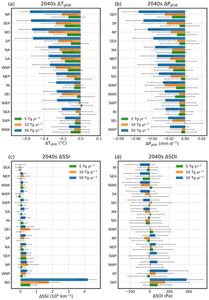
1. Length of simulations and ensemble size. Is 5 years long enough to spin up a fully coupled model and 10 years long enough to get a statistically significant signal? Time series of the global T and P response might help address whether the model is adequately spun up after 5 years. Additionally, in L211, do you mean the ERF responses in Figure 2? If so, the error bars on Fig.2 say standard error while Fig. 6 says standard deviation. If what is plotted indeed matches the captions, then it makes sense that the error in Fig. 6 would be smaller than Fig. 2. The authors should make the error calculation consistent between the plots to draw a fair comparison, as this is a key assumption that must be satisfied to warrant the methodology in the next set of simulations. Otherwise, I think that a few more ensemble members would be necessary to constrain the variability and robustness of the methodology. Given that there is high internal variability with concentrated regional scale perturbations, I’m not convinced that 1 ensemble member of a 10-year average is sufficient to truly develop a robust optimal strategy.
2. Linear additivity. While I can squint and convince myself that Fig. 3o and 3p look vaguely similar latitudinally, I find it much less convincing that there is agreement in the spatial patterns in Fig. 4o and 4p. While I do see traces of equatorial drying in the Atlantic, Indian, and West Pacific in both, the East Pacific drying in Fig. 4p is missing from 4o and almost all the moistening in the sum of regions is absent from the simultaneous simulation. The claim in L164-166 needs further justification given that the core methodology of this paper requires the linear additivity assumption to be satisfied. I agree with the statement in L236-237 that the climate responses are variable for the lower emission rates, but I am confused why scaling the response from the 50 Tg/y deployment would be a more robust proxy for smaller regional perturbations than 5 and 10 Tg/y simulations you’ve already run. Does this method “overcome the variability” in a physically realistic way? Would we expect the spatial pattern of responses to small perturbations to necessarily be scaled down versions of the response to larger perturbations (especially for hydrological variables)?
3. SOI climate response target. Targeting a mean value for T, P and SSI makes sense to me because there are clear increasing (T and P) and decreasing (SSI) trends for each of those variables (L269-270). It’s less clear that this target makes sense for SOI which is an oscillation. Is there a robust trend in SOI between 2015-2050 under global warming? Would a metric that captures changes magnitude and frequency separately be more appropriate for an oscillatory variable? For example, I could imagine a combination of patches that achieves the baseline mean SOI by decreasing the magnitude and frequency of El Niños in favor of La Niña conditions, which was described earlier in the paper as an unfavorable outcome. In other words, I wonder if this metric might measure a “successful” outcome for the wrong reasons. In Table 4, the delta SOI value for Optim-14 is wildly different from the Optim-6 and Midlat experiments and the farthest away from the target. Any speculation as to why this occurs? Could this be avoided by carefully selecting particular combinations from the 172 combinations rather than the mean to obtain the distribution? This is the only target that is missed with substantial error (error>mean) compared to the other targets but is not mentioned in the text. Failure modes of an “optimal” strategy are important to disclose and discuss. They could even give insight as to how to improve the methodology (either the formulation of the metric or selection of patches).
Minor comments
- L44-45: Should add reference to Xing et al. (2025) that explicitly analyzes the ENSO response to subtropical MCB (the authors find suppression of ENSO variability and a mean-state La Niña tendency).
References
Xing, C., Stevenson, S., Fasullo, J., Harrison, C., Chen, C., Wan, J., et al. (2025). Subtropical marine cloud brightening suppresses the El Niño–Southern Oscillation. Earth's Future, 13, e2025EF006522. https://doi.org/10.1029/2025EF006522
- L69: Maybe instead of “holistically” you could say “simultaneously”? Holistically is a bit vague since you arbitrarily chose a few large-scale climate metrics to analyze.
- L106-107: How do you define “open ocean”? Do you use a land/ocean mask? Is there further open ocean vs. coastal grid cell delineation? What is the % ocean area for the boxes (add column to Table 1)? Perhaps you could update Figure 1 to show the regions where SSA is injected (shading?) rather than boxes. I also think there is an extra box drawn between NP and WNP without a label (also shaded in the Optim-14 and Optim-6 experiments but doesn’t appear to be one of the 14 regions?).
- L119-120: Over what period are the 10-year transient AMIP simulations and what are the fixed SSTs?
- L140: What do you mean by pristine stratocumulus? The NEP is often considered a major stratocumulus cloud deck and the third region in early MCB studies, yet it does not have as strong of radiative forcing. It also appears that DRF dominates these stratocumulus regions, which is counter intuitive given the elevated low cloud fraction, while the SP and SA have the largest CRF response. Perhaps some maps of cloud fraction, cloud liquid water path and other related cloud properties would help.
- L152: I would make it clear here that you are transitioning away from the AMIP runs to the coupled simulations for the rest of the section/manuscript.
- L161: Are the +/- values one standard deviation? How were these errors calculated?
- L181-189: Why does NH MCB lead to an interhemispheric temperature imbalance but SH MCB does not? Looking at Fig. 5b, I would argue that SH MCB does influence the ITCZ position (otherwise it would be a bunch of flat lines), but there is no clear trend as in the NH MCB cases. In fact, the scale is larger on the y-axis in Fig. 5b than 5a, which suggests that the magnitude of changes (at least for SEP) are large just not coherent.
- L202-203: It seems important to note that most of the regions have an insignificant SSI response, even the 50 Tg/yr experiments (Fig. 6c). Only SA, WNP, and NO look like they have error bars that don’t cross 0, which is especially interesting since SA is one of the farthest seeding regions from the Arctic. How do you explain the mechanism for that result? Is the SA patch triggering a teleconnection in the Arctic?
- L204-205: Similar story with the SOI response—it appears that not only is the SEP the most sensitive, but it’s also the only statistically significant bar in Fig. 6d. Is this result sensitive to your choice in metric to quantify ENSO? For example, perhaps you could decompose the ENSO response into an oceanic (e.g. thermocline slope) and atmospheric (e.g., Walker Cell Index) component to get a clearer picture of the ENSO response?
- L224-227: It’s not clear from this text what delta T you are interpolating to get to 50 Tg/y. Maybe a figure would help visualize the interpolation. Referencing a future section (4.2) seems backwards. You should just describe what you want to say here first.
- L229-231: Why 10 x 5 Tg/y shares into some combination of the 14 regions? Is this aa computational constraint or other scientific rationale?
- Fig 7: should specify that the delta T and P are global mean over the 2040s?
- L273: Echoing the other reviewer, should NH/SH delta P should be climate response targets to capture changes in ITCZ shifts.
- L335: How are you calculating the correlation score? Are you comparing the 2040s mean MCB value vs 2014-2033 target (2 values per grid cell)? Or are there multiple ensemble members for these simulations?
- L390-395: Beyond other ESMs, more ensemble members and longer runs seem like necessary next steps for this work to interrogate uncertainty within the model itself. It’s also possible that more sophisticated optimization algorithms including AI could be useful for sampling different combinations of patches rather than this statistical approach.
Citation: https://doi.org/10.5194/egusphere-2025-5591-RC2 - AC1: 'Comment on egusphere-2025-5591', Alex M. Mason, 19 Mar 2026
- AC2: 'Comment on egusphere-2025-5591', Alex M. Mason, 19 Mar 2026
Peer review completion


Interactive discussion
Status: closed
-
RC1: 'Comment on egusphere-2025-5591', Anonymous Referee #1, 04 Jan 2026
General Comments
This manuscript presents a systematic and carefully constructed framework for designing multi-region MCB deployments based on a large ensemble of regional patch simulations using UKESM1.0. The optimization strategy—sampling and filtering over more than one million possible combinations using multiple climate response targets—is both novel and well motivated, and the comparison with a midlatitude-only deployment provides a useful benchmark within the existing MCB literature.
With revisions that more fully address the methodological limitations and clarify their implications, I believe this work would make a strong and valuable contribution to the literature on MCB deployment design.
Major Comments
- The paper’s central conclusions depend strongly on assumptions of linearity, additivity, and ERF-based scaling of coupled climate responses, which are not sufficiently stress-tested in the current analysis. While the optimized deployments are compelling as a proof-of-concept, the manuscript itself documents substantial nonlinearity and diminishing returns in ERF with increasing injection rate. These features raise important questions about the robustness of the scaling framework used to construct the optimized solutions. Equation (2) estimates the response of a MCB combination by scaling the 50 Tg yr-1 coupled responses using ERF ratios derived from fixed-SST simulations. While this approach is pragmatic, the manuscript does not justify why ERF(50 Tg yr-1) is used as the sole reference point, despite the availability of ERF estimates at 5 and 10 Tg yr-1. Although the authors note substantial variability in the coupled responses at 5 and 10 Tg yr-1, there is also appreciable variability at 50 Tg yr-1. Moreover, since most optimized combinations allocate only small fractions (5–10 Tg yr-1) to many regions, ERF(5 Tg yr-1) or ERF(10 Tg yr-1) may be more appropriate scaling references. Please consider a sensitivity test in which Eq. (2) is evaluated using ERF(5 Tg yr-1) or ERF(10 Tg yr-1) as the reference and discuss how the optimization results might change if the scaling reference were injection-rate dependent.
- The manuscript states that an MCB combination strategy should avoid seeding only the Northern Hemisphere in order to minimize southward ITCZ shifts and associated impacts on vulnerable regions such as South Asia and the Sahel. However, the optimization framework does not include an explicit ITCZ metric, nor does it constrain NH and SH precipitation (ΔP) separately as target variables. Is there a specific reason these metrics were not included? Given the strong allocation of MCB patches in the NH in the optimized deployments, it seems important to more directly incorporate hemispheric or ITCZ-related precipitation responses into the optimization targets.
Minor comments
- Line 119: According to Henry et al. (2025), sea-salt emissions in September in the NO are approximately twice as large as in other months, due to the seasonal maximum in open-ocean area. Given that the NO region plays a prominent role in the optimized deployments, it would be helpful to describe the seasonal variability more clearly in the main text, rather than only mentioning it briefly.
- Line 227: Including a simple figure would improve transparency and help readers better understand the rationale for selecting 50 Tg yr-1 as the reference deployment magnitude.
Technical corrections
- Line 190: It is unclear whether ΔT and ΔP refer to global-mean values. If so, please state this explicitly and ensure that the same convention is applied consistently throughout the manuscript.
- Line 211: “With comparison to the ERF responses in Figure 3…”. This appears to refer to Figure 2, which presents the ERF results. Please check and correct the figure numbering if necessary.
- Figure 8: For clarity, it would be helpful to note in the caption that the black arrows are arbitrary or conceptual, rather than representing specific quantitative values, as they could otherwise be misleading.
- Table 4: The reported value of ΔT for Optim-14 appears to be missing a minus sign. Please check and correct if necessary.
- Line 387: For clarity, please consider using a more explicit expression than “NO MCB” such as “MCB in the NO region” to improve readability for non-specialist readers.
Citation: https://doi.org/10.5194/egusphere-2025-5591-RC1 -
RC2: 'Comment on egusphere-2025-5591', Anonymous Referee #2, 15 Jan 2026
Summary
Mason et al. present a methodology for designing patchwork MCB strategies to optimize global climate targets in UKESM1.0. I believe this manuscript will be a valuable contribution to the field by systematically exploring the efficacy of different MCB regions that have been otherwise been somewhat arbitrarily chosen in the literature. I do have some questions regarding their methodology and analysis that should be addressed before publication.
Major comments
1. Length of simulations and ensemble size. Is 5 years long enough to spin up a fully coupled model and 10 years long enough to get a statistically significant signal? Time series of the global T and P response might help address whether the model is adequately spun up after 5 years. Additionally, in L211, do you mean the ERF responses in Figure 2? If so, the error bars on Fig.2 say standard error while Fig. 6 says standard deviation. If what is plotted indeed matches the captions, then it makes sense that the error in Fig. 6 would be smaller than Fig. 2. The authors should make the error calculation consistent between the plots to draw a fair comparison, as this is a key assumption that must be satisfied to warrant the methodology in the next set of simulations. Otherwise, I think that a few more ensemble members would be necessary to constrain the variability and robustness of the methodology. Given that there is high internal variability with concentrated regional scale perturbations, I’m not convinced that 1 ensemble member of a 10-year average is sufficient to truly develop a robust optimal strategy.
2. Linear additivity. While I can squint and convince myself that Fig. 3o and 3p look vaguely similar latitudinally, I find it much less convincing that there is agreement in the spatial patterns in Fig. 4o and 4p. While I do see traces of equatorial drying in the Atlantic, Indian, and West Pacific in both, the East Pacific drying in Fig. 4p is missing from 4o and almost all the moistening in the sum of regions is absent from the simultaneous simulation. The claim in L164-166 needs further justification given that the core methodology of this paper requires the linear additivity assumption to be satisfied. I agree with the statement in L236-237 that the climate responses are variable for the lower emission rates, but I am confused why scaling the response from the 50 Tg/y deployment would be a more robust proxy for smaller regional perturbations than 5 and 10 Tg/y simulations you’ve already run. Does this method “overcome the variability” in a physically realistic way? Would we expect the spatial pattern of responses to small perturbations to necessarily be scaled down versions of the response to larger perturbations (especially for hydrological variables)?
3. SOI climate response target. Targeting a mean value for T, P and SSI makes sense to me because there are clear increasing (T and P) and decreasing (SSI) trends for each of those variables (L269-270). It’s less clear that this target makes sense for SOI which is an oscillation. Is there a robust trend in SOI between 2015-2050 under global warming? Would a metric that captures changes magnitude and frequency separately be more appropriate for an oscillatory variable? For example, I could imagine a combination of patches that achieves the baseline mean SOI by decreasing the magnitude and frequency of El Niños in favor of La Niña conditions, which was described earlier in the paper as an unfavorable outcome. In other words, I wonder if this metric might measure a “successful” outcome for the wrong reasons. In Table 4, the delta SOI value for Optim-14 is wildly different from the Optim-6 and Midlat experiments and the farthest away from the target. Any speculation as to why this occurs? Could this be avoided by carefully selecting particular combinations from the 172 combinations rather than the mean to obtain the distribution? This is the only target that is missed with substantial error (error>mean) compared to the other targets but is not mentioned in the text. Failure modes of an “optimal” strategy are important to disclose and discuss. They could even give insight as to how to improve the methodology (either the formulation of the metric or selection of patches).
Minor comments
- L44-45: Should add reference to Xing et al. (2025) that explicitly analyzes the ENSO response to subtropical MCB (the authors find suppression of ENSO variability and a mean-state La Niña tendency).
References
Xing, C., Stevenson, S., Fasullo, J., Harrison, C., Chen, C., Wan, J., et al. (2025). Subtropical marine cloud brightening suppresses the El Niño–Southern Oscillation. Earth's Future, 13, e2025EF006522. https://doi.org/10.1029/2025EF006522
- L69: Maybe instead of “holistically” you could say “simultaneously”? Holistically is a bit vague since you arbitrarily chose a few large-scale climate metrics to analyze.
- L106-107: How do you define “open ocean”? Do you use a land/ocean mask? Is there further open ocean vs. coastal grid cell delineation? What is the % ocean area for the boxes (add column to Table 1)? Perhaps you could update Figure 1 to show the regions where SSA is injected (shading?) rather than boxes. I also think there is an extra box drawn between NP and WNP without a label (also shaded in the Optim-14 and Optim-6 experiments but doesn’t appear to be one of the 14 regions?).
- L119-120: Over what period are the 10-year transient AMIP simulations and what are the fixed SSTs?
- L140: What do you mean by pristine stratocumulus? The NEP is often considered a major stratocumulus cloud deck and the third region in early MCB studies, yet it does not have as strong of radiative forcing. It also appears that DRF dominates these stratocumulus regions, which is counter intuitive given the elevated low cloud fraction, while the SP and SA have the largest CRF response. Perhaps some maps of cloud fraction, cloud liquid water path and other related cloud properties would help.
- L152: I would make it clear here that you are transitioning away from the AMIP runs to the coupled simulations for the rest of the section/manuscript.
- L161: Are the +/- values one standard deviation? How were these errors calculated?
- L181-189: Why does NH MCB lead to an interhemispheric temperature imbalance but SH MCB does not? Looking at Fig. 5b, I would argue that SH MCB does influence the ITCZ position (otherwise it would be a bunch of flat lines), but there is no clear trend as in the NH MCB cases. In fact, the scale is larger on the y-axis in Fig. 5b than 5a, which suggests that the magnitude of changes (at least for SEP) are large just not coherent.
- L202-203: It seems important to note that most of the regions have an insignificant SSI response, even the 50 Tg/yr experiments (Fig. 6c). Only SA, WNP, and NO look like they have error bars that don’t cross 0, which is especially interesting since SA is one of the farthest seeding regions from the Arctic. How do you explain the mechanism for that result? Is the SA patch triggering a teleconnection in the Arctic?
- L204-205: Similar story with the SOI response—it appears that not only is the SEP the most sensitive, but it’s also the only statistically significant bar in Fig. 6d. Is this result sensitive to your choice in metric to quantify ENSO? For example, perhaps you could decompose the ENSO response into an oceanic (e.g. thermocline slope) and atmospheric (e.g., Walker Cell Index) component to get a clearer picture of the ENSO response?
- L224-227: It’s not clear from this text what delta T you are interpolating to get to 50 Tg/y. Maybe a figure would help visualize the interpolation. Referencing a future section (4.2) seems backwards. You should just describe what you want to say here first.
- L229-231: Why 10 x 5 Tg/y shares into some combination of the 14 regions? Is this aa computational constraint or other scientific rationale?
- Fig 7: should specify that the delta T and P are global mean over the 2040s?
- L273: Echoing the other reviewer, should NH/SH delta P should be climate response targets to capture changes in ITCZ shifts.
- L335: How are you calculating the correlation score? Are you comparing the 2040s mean MCB value vs 2014-2033 target (2 values per grid cell)? Or are there multiple ensemble members for these simulations?
- L390-395: Beyond other ESMs, more ensemble members and longer runs seem like necessary next steps for this work to interrogate uncertainty within the model itself. It’s also possible that more sophisticated optimization algorithms including AI could be useful for sampling different combinations of patches rather than this statistical approach.
Citation: https://doi.org/10.5194/egusphere-2025-5591-RC2 - AC1: 'Comment on egusphere-2025-5591', Alex M. Mason, 19 Mar 2026
- AC2: 'Comment on egusphere-2025-5591', Alex M. Mason, 19 Mar 2026
Peer review completion
Journal article(s) based on this preprint
Viewed
| HTML | XML | Total | BibTeX | EndNote | |
|---|---|---|---|---|---|
| 2,841 | 862 | 254 | 3,957 | 265 | 224 |
- HTML: 2,841
- PDF: 862
- XML: 254
- Total: 3,957
- BibTeX: 265
- EndNote: 224
Viewed (geographical distribution)
| Country | # | Views | % |
|---|
| Total: | 0 |
| HTML: | 0 |
| PDF: | 0 |
| XML: | 0 |
- 1

Matthew Henry
Haruki Hirasawa
Fiona M. O'Connor
James Haywood
The requested preprint has a corresponding peer-reviewed final revised paper. You are encouraged to refer to the final revised version.
- Preprint
(6077 KB) - Metadata XML
General Comments
This manuscript presents a systematic and carefully constructed framework for designing multi-region MCB deployments based on a large ensemble of regional patch simulations using UKESM1.0. The optimization strategy—sampling and filtering over more than one million possible combinations using multiple climate response targets—is both novel and well motivated, and the comparison with a midlatitude-only deployment provides a useful benchmark within the existing MCB literature.
With revisions that more fully address the methodological limitations and clarify their implications, I believe this work would make a strong and valuable contribution to the literature on MCB deployment design.
Major Comments
Minor comments
Technical corrections