
the Creative Commons Attribution 4.0 License.
the Creative Commons Attribution 4.0 License.
 | 27 Nov 2025
BiasCast: Learning and adjusting real time biases from meteorological forecasts to enhance runoff predictions
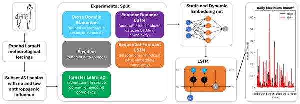
Abstract. The use of deep learning models in hydrology is becoming an ever more prevalent application in operational flood forecasting. Such operational systems face performance degradation when transitioning from high quality reanalysis to meteorological forecast data with lower accuracy. This study investigates training strategies and Long Short-Term Memory network architectures to mitigate forecast-induced bias in maximum daily discharge predictions using the Extended LamaH- CE dataset and a subset of 451 basins. We systematically evaluated cross-domain generalization, transfer learning approaches, Encoder–Decoder LSTMs, Sequential Forecast LSTMs, and the role of input embeddings and integrating past discharge observations. The results show that domain shifts between reanalysis and forecast data lead to substantial skill loss, with median Nash–Sutcliffe Efficiency decreasing from 0.58 to 0.33. Among the tested strategies, the Sequential Forecast LSTM demonstrated the most stable improvements, achieving a median NSE of 0.63. Integrating recent discharge observations further enhanced performance, raising median NSE to 0.71 and surpassing even the reanalysis-driven baseline. In contrast, integrating archived forecasts or using more complex input embeddings did not yield consistent benefits and in some cases degraded model stability. These findings highlight the value of training strategies that allow models to directly learn bias correction during forecast transitions and emphasize the operational potential of combining sequential processing with near real-time discharge observations.
-
Notice on discussion status
The requested preprint has a corresponding peer-reviewed final revised paper. You are encouraged to refer to the final revised version.
-
Preprint
(1571 KB)
-
The requested preprint has a corresponding peer-reviewed final revised paper. You are encouraged to refer to the final revised version.
- Preprint
(1571 KB) - Metadata XML
- BibTeX
- EndNote
- Final revised paper


Journal article(s) based on this preprint
Interactive discussion
Status: closed
-
RC1: 'Comment on egusphere-2025-4978', Anonymous Referee #1, 02 Jan 2026
-
AC1: 'Reply on RC1', Oliver Konold, 25 Mar 2026
We thank both anonymous referees for their careful reading of the manuscript and their detailed and constructive comments. We have carefully considered all comments and prepared point-by-point responses, which are attached as separate documents for Referee #1 and Referee #2.
-
AC1: 'Reply on RC1', Oliver Konold, 25 Mar 2026
-
RC2: 'Comment on egusphere-2025-4978', Anonymous Referee #2, 01 Mar 2026
Review of HESS Manuscript: “BiasCast: Learning and adjusting real time biases from meteorological forecasts to enhance runoff predictions”
Dear editor, please find attached my review of the manuscript.
1. Scope
The scope of the article is inside the scope of HESS.
2. Summary
The authors proposed methods to improve model performance under forecast-induced bias (performance drop when models trained on reanalysis data are used with forecast data). They test different strategies including encoder-decoder lstms, sequential-lstms and transfer learning. Moreover, they investigate how linear embeddings, and the inclusion of past-observed discharge influence performance.
3. General comments
I think the article is really well written, with a good introduction, clear objective and well-posed experiments. The results are presented in a clean way. Even with many model variations, it was easy to follow, which is not always the case. The only major limitation of the study is that the authors are limiting themselves to one-day-ahead prediction, when the LSTMs architectures and the available data already allow them to increase the lead times. This limits the conclusions that can be drawn, especially with the effect of decaying quality of the forecast as the lead time increases. From lines 95 and 489, I understand that this article is a stepping stone for multi-day prediction, so I understand that they want to leave that for a future study, but then they should clearly state this in the limitations section.
4. Specific comment
Line 139-142: It is good that you used embeddings, but this paragraph makes it sound as if an LSTM without embeddings cannot capture non-linear relationships nor learned how to combine the features, which they actually can. The main advantage of embeddings is that (1) you can reduce large input dimensions into smaller latten spaces, (2) the embeddings can learn to compensate for systematic bias in your data, for example if you use a different embedding for hindcast and forecast, and (3) if you use different type/groups of inputs with different number of variables, you can map them to a shared dimension for further processing (e.g Acuna2025 for multiple frequencies or Gauch2025 for missing data).
Line 146-148: I do not understand what you are trying to say, can you please rephrase or further explain?
Line 259-262: The problem with using tanh as the activation of the embeddings is that tanh saturates. Saturation is a known problem for lstms (Kratzert2024, Acuna2025, Baste2025), and I think it can be further increased if you also saturate the input before it goes into the LSTM. Was there a specific reason you used tanh? Have you tried if ReLu gives you better results, especially considering that in section 3.5 you indicate that more complex embeddings gave you worse performance for the enc-dec and seq-lstm. Are you using dropout in the more complex embeddings to avoid overfitting?
Section 3.1: Can you further explain the difference between BaseLine Reanalysis and CrossDomain (Reanalysis, Pretrain)?
Line 324-326: The sequential data processing is not only done in the sequential lstm, is it? I agree with what you said at the end of the paragraph, that sequential-lstm is better than encoder-decoder, because the hindcast-forecast transition is done on the same lstm instead of having to initialize a new one, especially in your case, where the forecast part is only run for one day. But this makes it sound like only the sequential-lstm process data sequentially and in temporal order, which is not true.
Line 435: The limitation of integrating reanalysis data depends on the test case. Multiple meteorological services have real-time observed data (from stations or radar), which is the data that can be included in the hindcast period, and then the forecast data comes from the meteorological models. I understand that if you are thinking on a global or continental scale, you might need reanalysis data, but in national-scale applications, you can directly use observed data (if the country has this available).
5. Recommendation
Dear editor, given the quality of the preprint, I recommend accepting it subject to minor revisions.
References:
Acuña Espinoza, E., Kratzert, F., Klotz, D., Gauch, M., Álvarez Chaves, M., Loritz, R., & Ehret, U. (2025). Technical note: An approach for handling multiple temporal frequencies with different input dimensions using a single LSTM cell. Hydrology and Earth System Sciences, 29(6), 1749–1758.
Acuña Espinoza, E., Loritz, R., Kratzert, F., Klotz, D., Gauch, M., Álvarez Chaves, M., & Ehret, U. (2025). Analyzing the generalization capabilities of a hybrid hydrological model for extrapolation to extreme events. Hydrology and Earth System Sciences, 29(5), 1277–1294. https://doi.org/10.5194/hess-29-1277-2025
Baste, S., Klotz, D., Acuña Espinoza, E., Bardossy, A., & Loritz, R. (2025). Unveiling the limits of deep learning models in hydrological extrapolation tasks. Hydrology and Earth System Sciences, 29(21), 5871–5891. https://doi.org/10.5194/hess-29-5871-2025
Gauch, M., Kratzert, F., Klotz, D., Nearing, G., Cohen, D., & Gilon, O. (2025). How to deal w___ missing input data. Hydrology and Earth System Sciences, 29(21), 6221–6235. https://doi.org/10.5194/hess-29-6221-2025
Kratzert, F., Gauch, M., Klotz, D., & Nearing, G. (2024). HESS Opinions: Never train a Long Short-Term Memory (LSTM) network on a single basin. Hydrology and Earth System Sciences, 28(17), 4187–4201. https://doi.org/10.5194/hess-28-4187-2024Citation: https://doi.org/10.5194/egusphere-2025-4978-RC2 -
AC2: 'Reply on RC2', Oliver Konold, 25 Mar 2026
We thank both anonymous referees for their careful reading of the manuscript and their detailed and constructive comments. We have carefully considered all comments and prepared point-by-point responses, which are attached as separate documents for Referee #1 and Referee #2.
-
AC2: 'Reply on RC2', Oliver Konold, 25 Mar 2026
Peer review completion


Interactive discussion
Status: closed
-
RC1: 'Comment on egusphere-2025-4978', Anonymous Referee #1, 02 Jan 2026
This manuscript addresses the challenge of deploying machine-learning hydrological models in operational forecasting by explicitly considering domain shift between reanalysis and forecast meteorological inputs. The authors explore alternative training strategies and LSTM architectures to improve 1-day streamflow forecasts, and the results suggest that architectures combining hindcast and forecast phases, which use reanalysis and forecast data respectively, provide the greatest performance gains. The study tackles an important problem, presents interesting results, and is structured well. Some additional analysis and clarifications would further strengthen the interpretation of the experiments and results.
General comments
- The paper would be greatly improved by further analysis on the variability of the skill across basins (please see comments 15 and 24 below). The manuscript emphasizes the impact of domain shift between reanalysis and forecast meteorological datasets; however, this shift is not spatially uniform across basins or meteorological variables. Further analysis of how variability in domain shift relates to basin-to-basin differences in model performance would strengthen the conclusions. In addition, the role of catchment attributes in modulating model skill is not discussed. Given the focus on a 1-day lead time, differences in hydrological response will strongly influence streamflow predictability and should be considered.
- The paper is largely framed in terms of mitigating biases in meteorological forecasts. However, the inclusion of near real-time streamflow observations (and to some extent the use of model architectures with hindcast-forecast phases) are likely reducing uncertainty associated with initial conditions and/or model structure. A slight adjustment to the framing, or an explicit discussion of the different uncertainty sources being addressed, would improve clarity (see comment 21).
Specific comments
- The introduction is well written and covers may aspects of the topic, but some of the motivations are incomplete.
- Lines 51-54: As the authors note, the focus on ECMWF-IFS data implies that the transferability of the method proposed by Han et al. (2021) to other NWP systems still needs to be tested. However, this limitation does not in itself imply that more robust bias-correction approaches are required, as suggested by the authors (“highlighting the need for more robust approaches”). The wording could be revised to reflect this distinction more clearly.
- Line 64: It is my understanding that errors in river discharge measurements are often localised (e.g., by vegetation growth or changes in the river channel, hydraulic disturbances near the gauge, etc)? Potentially the authors mean that river discharge observations are impacted by less spatial representativeness errors? Please clarify.
- Lines 72-74: The GloFAS forecasts are available across the globe so the comment “the quantile mapping correction is dependent on GloFAS forecasts, meaning it is not applicable for regions where no GloFAS forecast is available” may be misleading and should be clarified. The Hunt et al., (2022) method can also be applied to other distributed hydrological forecasts so is not dependent on GloFAS.
- Meteorological datasets:
- Section 2.1: It is not clear to me which meteorological variables and datasets are used. Are the E-OBS, MSWEP, and GLEAM datasets used? If so, in which experiments, and if not, please remove them from the discussion.
- Appendix A: Are all the variables in appendix A used? If so, I suggest adding a column to indicate which experiment they are used in, and if not, I suggest indicating this.
- Section 2.1: What is the distribution of observed timeseries available at each station? Do they all cover the full experimental period from 2003-2017:
- Line 122: Are nested catchments included within the 451 basins?
- Figure 2: It would be very helpful if this figure (or an additional figure) included a diagrammatic comparison of the model architectures, and, if possible, of the experiments performed.
- Line 141-142: For clarity, do the temporal splits contain the lookback window of 365-days such that the validation and testing is done over 2-years’ of forecasts (2011-2013 and 2015-2017, respectively) rather than 3 years?
- Line 160: “exclusively driven by reanalysis (e.g., ERA5) or spatially interpolated observational (e.g., E-OBS) data sources”. Does the RA baseline use ERA5 or E-OBS?
- Section 2.2.1/2.2.2: Which LSTM architecture is used for the baselines and the cross-domain experiments? Are they all multi-basin models (i.e., trained on all data)? Please clarify and include in the experimental figure (see comment 3).
- Line 230: I appreciate that the authors have kept the manuscript concise; however, since the premise of the paper is that differences between the reanalysis and forecast domains lead to errors, I feel that more discussion of these differences is needed. This could be addressed in a short additional section, or at minimum by adding text to Appendix B to guide readers on the key differences between the two domains.
- Line 243: Are the weights for the embedding of both the dynamic and static features updated or just the dynamic?
- Section 3: It would be useful to have a table that compares the statistics of each experiment. For example, in some sections the standard deviation is mentioned and in others it’s not. The interquartile range would also be an interesting statistic as the standard deviation is influenced a lot by the very worst performing stations.
- Figure 3: I’m struggling to understand this figure. From the experiment description I would expect there to be three lines: reanalysis baseline, forecast baseline, and the Cross domain where the model used for the reanalysis baseline is driven by forecast data in the test period. What is the difference between the “Cross Domain (Reanalysis, Pre train)” and the “Baseline Reanalysis”? It would be nice to see a discussion on the cause between the difference between the two, particularly as it seems to have a big impact on the worst performing basins. It would also be useful if the caption labels corresponded to the experiment description more directly.
- Section 3.1: It would strengthen the manuscript to explore the relationship between differences in meteorological reanalysis and forecast datasets and the resulting streamflow predictions. For example, do locations with the largest input differences show the greatest performance degradation in the cross-domain experiments?
- Figure 4:
- Are the arrows showing the median change in NSE or the change in median NSE (the caption suggests the former, but the arrows suggest the latter)? Please also check other figure captions for consistency.
- Also please check the 0.3 value associated with the orange line (Sequential Forecast LSTM) as it doesn’t seem consistent with the other values.
- Line 312: Interestingly, the difference between the two TL methods disappears at the 90th percentile. Can the authors explain this behaviour?
- Line 329: How many and what size layers does the handover network have, and are they tuned?
- Lines 335-336: I really like these summary sentences (e.g. “In short…”) at the start of each results section - very clear and helpful!
- Line 346: If pretrained with both reanalysis and forecast data as input, what is the model fine-tuned on? Is it the loss function that is changed rather than the inputs?
- Section 3.2/Section 3.4: The study focuses on training strategies and LSTM architectures to mitigate forecast-induced biases. However, the inclusion of near real-time streamflow observations may also be compensating for other uncertainties. A brief discussion of this effect would be helpful. Additionally, please justify the use of forecast- and reanalysis-based baselines as upper and lower benchmarks within this section (Seibert et al., 2018).
- Line 358: Where are the outliers? What is causing these outliers? For example, are they at high elevations? Do they have short observation records?
- Lines 380-381: “The Sequential Forecast LSTM exhibits even more impressive improvements when discharge is integrated, achieving a median NSE of 0.71 compared to 0.63 without discharge.” may be misleading because the improvement of the median NSE value is smaller than for the Encoder-decoder model despite it being for higher NSE values.
- Section 3.4: It would be useful to explore the relationship between catchment attributes and model performance, particularly since persistence methods can sometimes achieve high skill at a 1-day lead time. This would strengthen the results of the manuscript.
- Section 3.5: Please check throughout that the analysis of the graph is correct. For example, “In the baseline, encoder-decoder and sequential LSTM experiments, simple linear embedding networks produced slightly higher simulation performance compared to more complex embedding architectures.” (lines 409-411) but the dashed line (simple) is primarily to the left of the solid line (complex). I think there may also be an editing error in this section as the last paragraph seems to contradict the paragraph before.
- Section 3.6: Some relevant topics could be discussed further. For example,
- The study appears to use only ECMWF-HRES as the forecast dataset. While different resolutions are mentioned, how transferable are the results to other NWP systems?
- The analysis focuses on a 1-day lead time—how does this choice affect the interpretation and generalizability of the results?
- Static attributes are not discussed. How might they influence the results, particularly if static embedding networks are not fine-tuned in the TL experiments?
Technical corrections
- Line 11: Suggest using “meteorological-forecast-induced” for consistency with other section
- Line 32: “magnitudinal correct” should be “magnitude-correct” or “magnitudinally correct”
- Lines 146-148: Something is not quite right in the grammar of the sentence “Hereafter, we use …”. Please rewrite for clarity.
- Line 284: “with equal five” doesn’t make sense.
- Lines 583-584: This reference has no way of finding the dataset doi/url etc.
- Lines 454-456: Something is not quite right in the sentence beginning “The substantial improvements”. Please rephrase.
- Line 478: The Hunt et al method is not GloFAS-specific it is just applied to GloFAS but it does require an initial streamflow forecast.
- Appendix B: The orange colour is not defined in the caption
References
Seibert J, Vis MJP, Lewis E, van Meerveld HJ. Upper and lower benchmarks in hydrological modelling. Hydrological Processes. 2018; 32: 1120–1125. https://doi.org/10.1002/hyp.11476
Citation: https://doi.org/10.5194/egusphere-2025-4978-RC1 -
AC1: 'Reply on RC1', Oliver Konold, 25 Mar 2026
We thank both anonymous referees for their careful reading of the manuscript and their detailed and constructive comments. We have carefully considered all comments and prepared point-by-point responses, which are attached as separate documents for Referee #1 and Referee #2.
-
RC2: 'Comment on egusphere-2025-4978', Anonymous Referee #2, 01 Mar 2026
Review of HESS Manuscript: “BiasCast: Learning and adjusting real time biases from meteorological forecasts to enhance runoff predictions”
Dear editor, please find attached my review of the manuscript.
1. Scope
The scope of the article is inside the scope of HESS.
2. Summary
The authors proposed methods to improve model performance under forecast-induced bias (performance drop when models trained on reanalysis data are used with forecast data). They test different strategies including encoder-decoder lstms, sequential-lstms and transfer learning. Moreover, they investigate how linear embeddings, and the inclusion of past-observed discharge influence performance.
3. General comments
I think the article is really well written, with a good introduction, clear objective and well-posed experiments. The results are presented in a clean way. Even with many model variations, it was easy to follow, which is not always the case. The only major limitation of the study is that the authors are limiting themselves to one-day-ahead prediction, when the LSTMs architectures and the available data already allow them to increase the lead times. This limits the conclusions that can be drawn, especially with the effect of decaying quality of the forecast as the lead time increases. From lines 95 and 489, I understand that this article is a stepping stone for multi-day prediction, so I understand that they want to leave that for a future study, but then they should clearly state this in the limitations section.
4. Specific comment
Line 139-142: It is good that you used embeddings, but this paragraph makes it sound as if an LSTM without embeddings cannot capture non-linear relationships nor learned how to combine the features, which they actually can. The main advantage of embeddings is that (1) you can reduce large input dimensions into smaller latten spaces, (2) the embeddings can learn to compensate for systematic bias in your data, for example if you use a different embedding for hindcast and forecast, and (3) if you use different type/groups of inputs with different number of variables, you can map them to a shared dimension for further processing (e.g Acuna2025 for multiple frequencies or Gauch2025 for missing data).
Line 146-148: I do not understand what you are trying to say, can you please rephrase or further explain?
Line 259-262: The problem with using tanh as the activation of the embeddings is that tanh saturates. Saturation is a known problem for lstms (Kratzert2024, Acuna2025, Baste2025), and I think it can be further increased if you also saturate the input before it goes into the LSTM. Was there a specific reason you used tanh? Have you tried if ReLu gives you better results, especially considering that in section 3.5 you indicate that more complex embeddings gave you worse performance for the enc-dec and seq-lstm. Are you using dropout in the more complex embeddings to avoid overfitting?
Section 3.1: Can you further explain the difference between BaseLine Reanalysis and CrossDomain (Reanalysis, Pretrain)?
Line 324-326: The sequential data processing is not only done in the sequential lstm, is it? I agree with what you said at the end of the paragraph, that sequential-lstm is better than encoder-decoder, because the hindcast-forecast transition is done on the same lstm instead of having to initialize a new one, especially in your case, where the forecast part is only run for one day. But this makes it sound like only the sequential-lstm process data sequentially and in temporal order, which is not true.
Line 435: The limitation of integrating reanalysis data depends on the test case. Multiple meteorological services have real-time observed data (from stations or radar), which is the data that can be included in the hindcast period, and then the forecast data comes from the meteorological models. I understand that if you are thinking on a global or continental scale, you might need reanalysis data, but in national-scale applications, you can directly use observed data (if the country has this available).
5. Recommendation
Dear editor, given the quality of the preprint, I recommend accepting it subject to minor revisions.
References:
Acuña Espinoza, E., Kratzert, F., Klotz, D., Gauch, M., Álvarez Chaves, M., Loritz, R., & Ehret, U. (2025). Technical note: An approach for handling multiple temporal frequencies with different input dimensions using a single LSTM cell. Hydrology and Earth System Sciences, 29(6), 1749–1758.
Acuña Espinoza, E., Loritz, R., Kratzert, F., Klotz, D., Gauch, M., Álvarez Chaves, M., & Ehret, U. (2025). Analyzing the generalization capabilities of a hybrid hydrological model for extrapolation to extreme events. Hydrology and Earth System Sciences, 29(5), 1277–1294. https://doi.org/10.5194/hess-29-1277-2025
Baste, S., Klotz, D., Acuña Espinoza, E., Bardossy, A., & Loritz, R. (2025). Unveiling the limits of deep learning models in hydrological extrapolation tasks. Hydrology and Earth System Sciences, 29(21), 5871–5891. https://doi.org/10.5194/hess-29-5871-2025
Gauch, M., Kratzert, F., Klotz, D., Nearing, G., Cohen, D., & Gilon, O. (2025). How to deal w___ missing input data. Hydrology and Earth System Sciences, 29(21), 6221–6235. https://doi.org/10.5194/hess-29-6221-2025
Kratzert, F., Gauch, M., Klotz, D., & Nearing, G. (2024). HESS Opinions: Never train a Long Short-Term Memory (LSTM) network on a single basin. Hydrology and Earth System Sciences, 28(17), 4187–4201. https://doi.org/10.5194/hess-28-4187-2024Citation: https://doi.org/10.5194/egusphere-2025-4978-RC2 -
AC2: 'Reply on RC2', Oliver Konold, 25 Mar 2026
We thank both anonymous referees for their careful reading of the manuscript and their detailed and constructive comments. We have carefully considered all comments and prepared point-by-point responses, which are attached as separate documents for Referee #1 and Referee #2.
-
AC2: 'Reply on RC2', Oliver Konold, 25 Mar 2026
Peer review completion
Journal article(s) based on this preprint
Data sets
Experimental Setups and Results for "BiasCast: Learning and adjusting real time biases from meteorological forecasts to enhance runoff predictions" Oliver Konold et al. https://doi.org/10.5281/zenodo.17241922
Extended LamaH-CE: LArge-SaMple DAta for Hydrology and Environmental Sciences for Central Europe Oliver Konold et al. https://doi.org/10.5281/zenodo.17119634
Model code and software
Forked NeuralHydrology Version Oliver Konold https://github.com/conestone/neuralhydrology
Interactive computing environment
Experiments and Results Code for "BiasCast: Learning and adjusting real time biases from meteorological forecasts to enhance runoff predictions" Oliver Konold https://github.com/conestone/biascast
Viewed
| HTML | XML | Total | BibTeX | EndNote | |
|---|---|---|---|---|---|
| 2,029 | 1,825 | 147 | 4,001 | 666 | 1,348 |
- HTML: 2,029
- PDF: 1,825
- XML: 147
- Total: 4,001
- BibTeX: 666
- EndNote: 1,348
Viewed (geographical distribution)
| Country | # | Views | % |
|---|
| Total: | 0 |
| HTML: | 0 |
| PDF: | 0 |
| XML: | 0 |
- 1
Cited



Moritz Feigl
Patrick Podest
Christoph Klingler
Karsten Schulz
The requested preprint has a corresponding peer-reviewed final revised paper. You are encouraged to refer to the final revised version.
- Preprint
(1571 KB) - Metadata XML
This manuscript addresses the challenge of deploying machine-learning hydrological models in operational forecasting by explicitly considering domain shift between reanalysis and forecast meteorological inputs. The authors explore alternative training strategies and LSTM architectures to improve 1-day streamflow forecasts, and the results suggest that architectures combining hindcast and forecast phases, which use reanalysis and forecast data respectively, provide the greatest performance gains. The study tackles an important problem, presents interesting results, and is structured well. Some additional analysis and clarifications would further strengthen the interpretation of the experiments and results.
General comments
Specific comments
Technical corrections
References
Seibert J, Vis MJP, Lewis E, van Meerveld HJ. Upper and lower benchmarks in hydrological modelling. Hydrological Processes. 2018; 32: 1120–1125. https://doi.org/10.1002/hyp.11476