
the Creative Commons Attribution 4.0 License.
the Creative Commons Attribution 4.0 License.
 | 05 Mar 2026
Quantifying national, state, and oil/gas field methane emissions and trends in the U.S. (2019–2024) through high resolution inversion of satellite observations
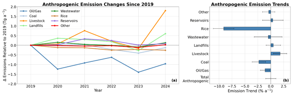
Abstract. We quantify trends of U.S. methane emissions at the national, state, and oil/gas field levels for 2019–2024 through high-resolution (up to ~25 km) analytical inversion of TROPOMI satellite observations with the open-source Integrated Methane Inversion (IMI 2.1). We find that total anthropogenic methane emissions (37 Tg a-1) are 34 % higher in magnitude than reported in the U.S. Environmental Protection Agency (EPA) Greenhouse Gas Inventory (GHGI) that provided prior estimates for the inversion. Oil/gas emissions are 64 % higher than the GHGI, consistent with previous studies. Total emissions are flat over the 2019–2024 period (0.0 ± 1.0 % a-1) but this total reflects a combination of decreasing emissions from the oil/gas (-1.1 ± 0.9 % a-1), coal (-2.3 ± 1.3 % a-1), and rice (-9.1 % ± 2.0 a-1) sectors, offset by increases in the livestock (1.8 ± 1.3 % a-1) and landfill (0.5 ± 1.4 % a-1) sectors. The methane intensity from the oil/gas sector continues its downward trend, from 2.3 % to 1.9 % over the 2019–2024 period, but unlike in previous studies we find that this trend does not simply reflect an increase in production but also a decrease in emissions, demonstrating improved emission management. Over half of total U.S. emissions originate from ten states, most dominated by fuel exploitation. Emission inventories compiled by individual states do not always improve on GHGI state estimates. Methane intensities decrease for all major oil/gas fields except those with declining production.
-
Notice on discussion status
The requested preprint has a corresponding peer-reviewed final revised paper. You are encouraged to refer to the final revised version.
-
Preprint
(1672 KB)
-
Supplement
(520 KB)
-
The requested preprint has a corresponding peer-reviewed final revised paper. You are encouraged to refer to the final revised version.
- Preprint
(1672 KB) - Metadata XML
-
Supplement
(520 KB) - BibTeX
- EndNote
- Final revised paper


Journal article(s) based on this preprint
Interactive discussion
Status: closed
- RC1: 'Comment on egusphere-2026-655', Anonymous Referee #1, 14 May 2026
-
RC2: 'Comment on egusphere-2026-655', Anonymous Referee #2, 05 Jun 2026
Review of "Quantifying national, state, and oil/gas field methane emissions and trends in the U.S. (2019-2024) through high resolution inversion of satellite observations" by Estrada et al., for ACP.
Overall notes: This manuscript describes a modeling study to quantify emissions and multi-year trends of methane over the continental US. There have been many similar studies in the past (many from this same team), but this study combines a higher spatial resolution analysis with multiple years. It also updates the trends relative to other papers, showing a continued decline in overall anthropogenic emissions. It is a well-written document and consists of a thorough high-quality analysis. The sector-based attribution of emissions however is based only on the prior emissions, and while this is noted in the manuscript, it would be nice to see some comments on how this affects the final conclusions in terms of the uncertainty of sectoral attribution. I also visited the custom dashboard and was very impressed - this is the kind of data scientists should be providing to policy makers directly, with state-level emissions provided for multiple years, and easily understood and downloaded.
Specific comments:
L120, super-observations are mentioned here before being defined later in the text. I would even advocate for a separate sub-section on observations and background rather than jumping right into the inversion method, even if it is only a few sentences, just so the reader can quickly understand what observations are being used and how they are averaged, etc. Also, including information about how the observations were averaged into super-observations without requiring the reader to go to another reference would be nice.
L147, here the optimization of the background is mentioned without noting what the prior background condition was, that is stated later in the text. Again, this could go into the same section as the observation detail.
L154: Can the authors comment on how the uncertainty on the trend would differ if it were calculated for each separate inversion and then averaged across the inversions? i.e. this trend does not incorporate the uncertainty from inversion method or use the spread from the 42 inversions in any way, correct?
Table 1: How were the values in Table 1 obtained, e.g., the 10 ppb error on the boundary condition, or the observational error standard deviation. Does the observational error standard deviation include transport uncertainty estimate? How are the values of the regularization parameter obtained (gamma)?
L193: How does the assumption of the sectoral attribution of the prior for each cell affect the conclusions of the study as it relates to oil and gas? is this uncertainty incorporated at all into the formal uncertainties for each sector? (presumably for many gas basins the uncertainty is small, where there are no other co-located large methane sources and the prior sectoral attribution is likely more robust)?
L227: Were posterior estimates only aggregated annually, with no further temporal resolution? Recent studies have pointed to possible seasonality in fossil methane emissions (Hu et al., ES&T), is any such seasonality possible to be determined in this study? Are observations sampled equally across seasons, or is there any seasonality to the availability of observations that may skew the annual result? (i.e. if emissions really are seasonal, would this cause aggregation error in the annual posterior estimates?)
L283: It is not clear to me why the lack of correlation with head count points to manure management as the source of this trend, likely because I am not as familiar with what governs emissions from this sector -- perhaps connect these dots for the reader?
L320: Why specifically was Colorado included? (perhaps just a sentence?) Is it because of the target on emissions they have set?
Citation: https://doi.org/10.5194/egusphere-2026-655-RC2 -
RC3: 'Comment on egusphere-2026-655', Andrew Schuh, 29 Jun 2026
Review:
We commend the authors for a well written and comprehensive manuscript. They find that, overall, CH4 emissions are about 34% higher than given by the EPA’s GHG inventory, but have little overall annual trend over the 2019-2024 period due to offsetting trends at the sectoral level. The methodology allows for and provides very interesting results and evaluation both at individual states and oil & gas basins, giving additional opportunities for comparison to state inventories and independent estimates of basin-level emissions.
We note that increasingly flux inversion systems are being packaged into tools such as the Integrated Methane Inversion (IMI) framework, making characterization of the details of the inversion much more opaque. That being said, the framework has been robustly developed for many years for CH4, in particular for TROPOMI XCH4 observations and we feel confident in its use here. The lead author wrote the IMI 2.0 manuscript and this paper appears to be the first step application of that system to recent CH4 data. We note that the visualization tool that is referenced in the conclusions is very nice too ( https://laestrada.github.io/ ).
General Comments:
- The IMI, essentially being a regional analytical inversion framework, should provide some kind of closed form posterior covariance/correlation information (matrix). There seems to be a few places where this could come into play in this manuscript but doesn’t?
- First, the authors note a large mean bias in annual CH4 emissions across the time region of interest but almost no trend in that number. Surprisingly there seems to be some significant sectoral adjustments as well as sectoral trends evident with the total emissions? It would seem interesting to me, and maybe others, to quantify the correlation structures between the sector estimates? While the analytical correlations may be hard to compute, a simple Monte Carlo draw from the posterior covariance, applied to flux fields would probably give you a sample covariance/correlation? I would anticipate very strong correlation (or anti-correlation) structure across the sector estimates? Even some exploratory calculations to verify/refute this and then comment would be great.
- The authors note that regions were split across state boundaries in order to aggregate geopolitically. It might be worth pointing out in the text that state estimate uncertainties are essentially ‘marginal standard deviations’ in that they don’t account for other nearby emissions. Each state can have a higher uncertainty while the sum is more constrained. Permian is a good example as discussed below in (4).
- Having done regional CO2 flux inversion work over North America in the past, I recall boundary inflow being a possible sensitivity, particularly in the southern boundary for CONUS, and possibly feeding into the Permian area. I noticed that you only present annual flux estimates, have you looked at seasonal fluxes? Particularly for differences in flux estimates seasonally? And if they exist, whether they are likely tied to emissions or possibly differing transport patterns pulling in boundary conditions?
- I would like to ask for one thing here. As part of my aforementioned regional CO2 flux work in 2010s, we also considered boundary inflow corrections similar to Nesser et al 2025. While I’m uncertain whether this needs to be in the manuscript, can you provide some figures of what the corrections look like? I’m curious, and others might be as well. That boundary inflow dual optimization can be a tricky thing to do in practice I found.
- I would like to ask you to consider adding a short note on uncertainty in the paper, both for completeness and for educational purposes? You present a map of marginal AK values in Fig 1d, then aggregate these spatial pieces up into national, state, and field level emissions numbers. It would be great to put in a couple sentences around section 3.1, just reminding readers of the fact that aggregation in this fashion is likely reducing uncertainty across the sum. The fact that the Permian is split across NM and TX is probably a great example and I’m guessing the uncertainty on the summed field level emissions should be less than the sum of the individual uncertainties. This is a nice additional justification for your aggregation by oil/gas region. Again, not absolutely required as you’re doing things correct here, but an opportunity to emphasize to readers the need for proper aggregation of posterior uncertainty as you are doing here.
On the National and state-level comparisons, We have some additional comments:
1) Table 1 is providing a comparison of the inversion results to the 2017-20 GHGI. While we understand this is the prior used in the inversion (or at least the 2019-20 EE is), the imperfect overlap in the time period does limit the available conclusions that can be made as more recent data is available. Is it possible to make a comparison to the recently released GHGIA (https://ghgi.cgs.umd.edu/) which covers through 2024 to evaluate whether the inventories and satellites are at least seeing similar sectoral-level trends, despite the significantly larger emissions from the inversion result? We know that this cannot be further allocated down to the state level as the Gridded GHGI has yet to be updated, yet this still provides a valuable point of comparison to the same time period.
2) The stacked line graphs of the left graph on Figure 3 make it very challenging to discern the relative contributions of each sector, can this be shown as a line graph (or several subplots on different axes scales if needed for clarity) to make it more clear to the reader how the different sectors are trending per year. Related to #1 above, It would also be interesting to see how these compare to the GHGIA trends.
3) Can manure management and enteric fermentation estimates be separately investigated to test the hypothesis proposed ~L245, or the state-level discussions ~L280? While they are often co-located, Pg S9 of the Maasakkers et al 2022 publication indicates a quite significant differences in spatial distribution in the two sources as used in your prior.
4) While rice agriculture is a large decreasing trend, it is also decreasing in the Maasakkers et al inventory from 2012-2018, and its large percentage is partially inflated by being the smallest categorical sector as broken out in this work. That could be worth a mention.
5) Regarding the claim on L262-3, can this be visualized side-by side by showing total emissions from this and other studies alongside the intensity in Fig 4?
6) Texas produced their first ever GHG inventory last year - given its contribution as the highest emitting state, it would be worthwhile to include this within the available state-level comparisons and discussions (see link to documents and data here: https://www.tceq.texas.gov/agency/climate-pollution-reduction-grants).
7) Varon et al 2025 does corroborate the results in New Mexico over a similar time period, this is fundamentally not surprising since that study is also performing an inversion of TROPOMI data via IMI (although there are some slight differences in methods). An additional citation for this from entirely independent aerial survey results can be confirmed between that of Shen et al 2022 (https://pubs.acs.org/doi/10.1021/acs.est.1c06458) and Donahue et al 2026 (https://doi.org/10.1021/acs.est.5c15184).
8) While the statement on line 321 is accurate (50% total GHG reduction reduction by 2030), the subsequent statements only address the O&G sector and not the other rules and regulations including Landfills, industrial, manufacturing and Transportation sectors (Details here under ‘Adopted rules’: https://cdphe.colorado.gov/apcd/climatechange). Recommend making this more clear, or adding a clause about either O&G specific targets or the statements being O&G sector specific actions. Additionally, Colorado published an updated greenhouse gas inventory in early 2026, significantly downscaling the O&G sector CH4 emissions from the prior inventory currently cited (https://cdphe.colorado.gov/apcd/greenhouse-gas-inventory).
Minor Comments
1) Recommend the use of ‘segment’ rather than ‘scope’ on Figure S3.
#####
Joint review by Dr. Andrew Schuh (Colorado State University) & Dr. Ben Hmiel (CD
Citation: https://doi.org/10.5194/egusphere-2026-655-RC3 - AC1: 'Comment on egusphere-2026-655', Lucas Estrada, 07 Jul 2026
Peer review completion


Interactive discussion
Status: closed
-
RC1: 'Comment on egusphere-2026-655', Anonymous Referee #1, 14 May 2026
General comments:
Estrada et al. present the results of a series of annual optimizations of methane emissions in the continental U.S. using TROPOMI satellite retrievals. This is a key progression from previous satellite inversions of methane emissions in the U.S. that were more limited in horizontal resolution, spatial extent, or time range. The manuscript is written clearly and presents external validation of methane emissions by sector at national and sub-national scales alongside an easily accessible online visualization tool, demonstrating the utility of their software for informing efforts to mitigate methane emissions in the U.S. and beyond. The work would benefit from some additional detail on a couple of their assumptions and comparisons, but overall, this is an impactful contribution to the ongoing discussion of methane emissions in scientific and policy communities.
Specific comments:
- Page 4, Figure 1: Averaging kernel sensitivities are shown here, and aggregated by state in Table S1, but are not discussed in the text beyond a definition in Section 2.1. Readers without a background in inverse modeling would benefit from interpretation of where your methods struggle to constrain emissions. Are there locations or sectors whose posterior results may be biased by consistently low sensitivity? Is sensitivity in 2024 representative of the full six years?
- Page 7, lines 196-197: To show that this is sufficient for attributing emissions by sector with reasonable accuracy, it would be helpful to include some analysis of co-located emissions and their potential impact on posterior trends or sectoral totals, particularly for smaller sources like rice and U.S. states with relatively few state vector elements like in New England and the Pacific Northwest.
- Page 7-8, lines 209-210: Is there any spatial pattern in prior bias, posterior bias, or change in bias when comparing to NOAA sites? Does it match Fig. 2a,b?
- Page 8, lines 224-225: There are some differences worth mentioning here in emissions from livestock and coal. Also, how do CONUS totals compare with other studies? It may be interesting to see some of the results in Figure S1 in a format similar to Figure 4 as well. Do the results of previous studies alongside your work show any trend?
Technical corrections:
- Table S1: Check units on rightmost column (sensitivity)
Citation: https://doi.org/10.5194/egusphere-2026-655-RC1 -
RC2: 'Comment on egusphere-2026-655', Anonymous Referee #2, 05 Jun 2026
Review of "Quantifying national, state, and oil/gas field methane emissions and trends in the U.S. (2019-2024) through high resolution inversion of satellite observations" by Estrada et al., for ACP.
Overall notes: This manuscript describes a modeling study to quantify emissions and multi-year trends of methane over the continental US. There have been many similar studies in the past (many from this same team), but this study combines a higher spatial resolution analysis with multiple years. It also updates the trends relative to other papers, showing a continued decline in overall anthropogenic emissions. It is a well-written document and consists of a thorough high-quality analysis. The sector-based attribution of emissions however is based only on the prior emissions, and while this is noted in the manuscript, it would be nice to see some comments on how this affects the final conclusions in terms of the uncertainty of sectoral attribution. I also visited the custom dashboard and was very impressed - this is the kind of data scientists should be providing to policy makers directly, with state-level emissions provided for multiple years, and easily understood and downloaded.
Specific comments:
L120, super-observations are mentioned here before being defined later in the text. I would even advocate for a separate sub-section on observations and background rather than jumping right into the inversion method, even if it is only a few sentences, just so the reader can quickly understand what observations are being used and how they are averaged, etc. Also, including information about how the observations were averaged into super-observations without requiring the reader to go to another reference would be nice.
L147, here the optimization of the background is mentioned without noting what the prior background condition was, that is stated later in the text. Again, this could go into the same section as the observation detail.
L154: Can the authors comment on how the uncertainty on the trend would differ if it were calculated for each separate inversion and then averaged across the inversions? i.e. this trend does not incorporate the uncertainty from inversion method or use the spread from the 42 inversions in any way, correct?
Table 1: How were the values in Table 1 obtained, e.g., the 10 ppb error on the boundary condition, or the observational error standard deviation. Does the observational error standard deviation include transport uncertainty estimate? How are the values of the regularization parameter obtained (gamma)?
L193: How does the assumption of the sectoral attribution of the prior for each cell affect the conclusions of the study as it relates to oil and gas? is this uncertainty incorporated at all into the formal uncertainties for each sector? (presumably for many gas basins the uncertainty is small, where there are no other co-located large methane sources and the prior sectoral attribution is likely more robust)?
L227: Were posterior estimates only aggregated annually, with no further temporal resolution? Recent studies have pointed to possible seasonality in fossil methane emissions (Hu et al., ES&T), is any such seasonality possible to be determined in this study? Are observations sampled equally across seasons, or is there any seasonality to the availability of observations that may skew the annual result? (i.e. if emissions really are seasonal, would this cause aggregation error in the annual posterior estimates?)
L283: It is not clear to me why the lack of correlation with head count points to manure management as the source of this trend, likely because I am not as familiar with what governs emissions from this sector -- perhaps connect these dots for the reader?
L320: Why specifically was Colorado included? (perhaps just a sentence?) Is it because of the target on emissions they have set?
Citation: https://doi.org/10.5194/egusphere-2026-655-RC2 -
RC3: 'Comment on egusphere-2026-655', Andrew Schuh, 29 Jun 2026
Review:
We commend the authors for a well written and comprehensive manuscript. They find that, overall, CH4 emissions are about 34% higher than given by the EPA’s GHG inventory, but have little overall annual trend over the 2019-2024 period due to offsetting trends at the sectoral level. The methodology allows for and provides very interesting results and evaluation both at individual states and oil & gas basins, giving additional opportunities for comparison to state inventories and independent estimates of basin-level emissions.
We note that increasingly flux inversion systems are being packaged into tools such as the Integrated Methane Inversion (IMI) framework, making characterization of the details of the inversion much more opaque. That being said, the framework has been robustly developed for many years for CH4, in particular for TROPOMI XCH4 observations and we feel confident in its use here. The lead author wrote the IMI 2.0 manuscript and this paper appears to be the first step application of that system to recent CH4 data. We note that the visualization tool that is referenced in the conclusions is very nice too ( https://laestrada.github.io/ ).
General Comments:
- The IMI, essentially being a regional analytical inversion framework, should provide some kind of closed form posterior covariance/correlation information (matrix). There seems to be a few places where this could come into play in this manuscript but doesn’t?
- First, the authors note a large mean bias in annual CH4 emissions across the time region of interest but almost no trend in that number. Surprisingly there seems to be some significant sectoral adjustments as well as sectoral trends evident with the total emissions? It would seem interesting to me, and maybe others, to quantify the correlation structures between the sector estimates? While the analytical correlations may be hard to compute, a simple Monte Carlo draw from the posterior covariance, applied to flux fields would probably give you a sample covariance/correlation? I would anticipate very strong correlation (or anti-correlation) structure across the sector estimates? Even some exploratory calculations to verify/refute this and then comment would be great.
- The authors note that regions were split across state boundaries in order to aggregate geopolitically. It might be worth pointing out in the text that state estimate uncertainties are essentially ‘marginal standard deviations’ in that they don’t account for other nearby emissions. Each state can have a higher uncertainty while the sum is more constrained. Permian is a good example as discussed below in (4).
- Having done regional CO2 flux inversion work over North America in the past, I recall boundary inflow being a possible sensitivity, particularly in the southern boundary for CONUS, and possibly feeding into the Permian area. I noticed that you only present annual flux estimates, have you looked at seasonal fluxes? Particularly for differences in flux estimates seasonally? And if they exist, whether they are likely tied to emissions or possibly differing transport patterns pulling in boundary conditions?
- I would like to ask for one thing here. As part of my aforementioned regional CO2 flux work in 2010s, we also considered boundary inflow corrections similar to Nesser et al 2025. While I’m uncertain whether this needs to be in the manuscript, can you provide some figures of what the corrections look like? I’m curious, and others might be as well. That boundary inflow dual optimization can be a tricky thing to do in practice I found.
- I would like to ask you to consider adding a short note on uncertainty in the paper, both for completeness and for educational purposes? You present a map of marginal AK values in Fig 1d, then aggregate these spatial pieces up into national, state, and field level emissions numbers. It would be great to put in a couple sentences around section 3.1, just reminding readers of the fact that aggregation in this fashion is likely reducing uncertainty across the sum. The fact that the Permian is split across NM and TX is probably a great example and I’m guessing the uncertainty on the summed field level emissions should be less than the sum of the individual uncertainties. This is a nice additional justification for your aggregation by oil/gas region. Again, not absolutely required as you’re doing things correct here, but an opportunity to emphasize to readers the need for proper aggregation of posterior uncertainty as you are doing here.
On the National and state-level comparisons, We have some additional comments:
1) Table 1 is providing a comparison of the inversion results to the 2017-20 GHGI. While we understand this is the prior used in the inversion (or at least the 2019-20 EE is), the imperfect overlap in the time period does limit the available conclusions that can be made as more recent data is available. Is it possible to make a comparison to the recently released GHGIA (https://ghgi.cgs.umd.edu/) which covers through 2024 to evaluate whether the inventories and satellites are at least seeing similar sectoral-level trends, despite the significantly larger emissions from the inversion result? We know that this cannot be further allocated down to the state level as the Gridded GHGI has yet to be updated, yet this still provides a valuable point of comparison to the same time period.
2) The stacked line graphs of the left graph on Figure 3 make it very challenging to discern the relative contributions of each sector, can this be shown as a line graph (or several subplots on different axes scales if needed for clarity) to make it more clear to the reader how the different sectors are trending per year. Related to #1 above, It would also be interesting to see how these compare to the GHGIA trends.
3) Can manure management and enteric fermentation estimates be separately investigated to test the hypothesis proposed ~L245, or the state-level discussions ~L280? While they are often co-located, Pg S9 of the Maasakkers et al 2022 publication indicates a quite significant differences in spatial distribution in the two sources as used in your prior.
4) While rice agriculture is a large decreasing trend, it is also decreasing in the Maasakkers et al inventory from 2012-2018, and its large percentage is partially inflated by being the smallest categorical sector as broken out in this work. That could be worth a mention.
5) Regarding the claim on L262-3, can this be visualized side-by side by showing total emissions from this and other studies alongside the intensity in Fig 4?
6) Texas produced their first ever GHG inventory last year - given its contribution as the highest emitting state, it would be worthwhile to include this within the available state-level comparisons and discussions (see link to documents and data here: https://www.tceq.texas.gov/agency/climate-pollution-reduction-grants).
7) Varon et al 2025 does corroborate the results in New Mexico over a similar time period, this is fundamentally not surprising since that study is also performing an inversion of TROPOMI data via IMI (although there are some slight differences in methods). An additional citation for this from entirely independent aerial survey results can be confirmed between that of Shen et al 2022 (https://pubs.acs.org/doi/10.1021/acs.est.1c06458) and Donahue et al 2026 (https://doi.org/10.1021/acs.est.5c15184).
8) While the statement on line 321 is accurate (50% total GHG reduction reduction by 2030), the subsequent statements only address the O&G sector and not the other rules and regulations including Landfills, industrial, manufacturing and Transportation sectors (Details here under ‘Adopted rules’: https://cdphe.colorado.gov/apcd/climatechange). Recommend making this more clear, or adding a clause about either O&G specific targets or the statements being O&G sector specific actions. Additionally, Colorado published an updated greenhouse gas inventory in early 2026, significantly downscaling the O&G sector CH4 emissions from the prior inventory currently cited (https://cdphe.colorado.gov/apcd/greenhouse-gas-inventory).
Minor Comments
1) Recommend the use of ‘segment’ rather than ‘scope’ on Figure S3.
#####
Joint review by Dr. Andrew Schuh (Colorado State University) & Dr. Ben Hmiel (CD
Citation: https://doi.org/10.5194/egusphere-2026-655-RC3 - AC1: 'Comment on egusphere-2026-655', Lucas Estrada, 07 Jul 2026
Peer review completion
Journal article(s) based on this preprint
Viewed
| HTML | XML | Total | Supplement | BibTeX | EndNote | |
|---|---|---|---|---|---|---|
| 1,757 | 1,021 | 124 | 2,902 | 308 | 163 | 186 |
- HTML: 1,757
- PDF: 1,021
- XML: 124
- Total: 2,902
- Supplement: 308
- BibTeX: 163
- EndNote: 186
Viewed (geographical distribution)
| Country | # | Views | % |
|---|
| Total: | 0 |
| HTML: | 0 |
| PDF: | 0 |
| XML: | 0 |
- 1

Daniel J. Jacob
James D. East
Daniel J. Varon
Nicholas Balasus
Sarah E. Hancock
Melissa Sulprizio
Kevin W. Bowman
John R. Worden
Emily Reidy
Benjamin R. K. Runkle
The requested preprint has a corresponding peer-reviewed final revised paper. You are encouraged to refer to the final revised version.
- Preprint
(1672 KB) - Metadata XML
-
Supplement
(520 KB) - BibTeX
- EndNote
- Final revised paper
General comments:
Estrada et al. present the results of a series of annual optimizations of methane emissions in the continental U.S. using TROPOMI satellite retrievals. This is a key progression from previous satellite inversions of methane emissions in the U.S. that were more limited in horizontal resolution, spatial extent, or time range. The manuscript is written clearly and presents external validation of methane emissions by sector at national and sub-national scales alongside an easily accessible online visualization tool, demonstrating the utility of their software for informing efforts to mitigate methane emissions in the U.S. and beyond. The work would benefit from some additional detail on a couple of their assumptions and comparisons, but overall, this is an impactful contribution to the ongoing discussion of methane emissions in scientific and policy communities.
Specific comments:
Technical corrections: