
the Creative Commons Attribution 4.0 License.
the Creative Commons Attribution 4.0 License.
 | 19 Jun 2026
When the Comparison Is the Problem: Spatial Resolution and Validation Bias in InSAR-Derived Coastal Subsidence Assessments Along the U.S. Gulf Coast
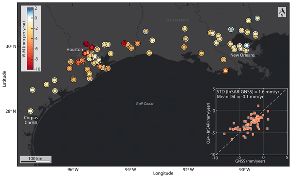
Abstract. Li et al. (2026) compare two InSAR-derived surface-elevation change datasets for the central U.S. Gulf Coast and conclude that InSAR is unreliable in vegetated coastal settings for rates below 5 mm/yr. While InSAR reproducibility is a timely and consequential question, we demonstrate that the paper's principal conclusions rest on three methodological decisions that critically undermine the comparison: (1) spatial aggregation of the O24 dataset from its native 50 m to 1 km prior to comparison, a ~400x reduction in pixel density that destroys the sub-kilometer spatial structure for which the dataset was designed; (2) a progressively filtered GNSS validation network of only ~20 stations concentrated in atypical stable Pleistocene upland settings, contrasting with O24's original validation across 157 stations spanning the full coastal domain; and (3) a 5 mm/yr caution threshold derived from inter-product disagreement between two methodologically dissimilar datasets rather than from principled uncertainty quantification. We validate O24 at its native 50 m resolution against 88 GNSS stations from the Nevada Geodetic Laboratory within the Li et al. study domain, obtaining a residual standard deviation of 1.6 mm/yr, consistent with Ohenhen et al. (2024) and directly contradicting the paper's characterization of O24 performance. We call on the InSAR community to prioritize coordinated benchmarking and invest in methodological literacy around resolution, coherence, and uncertainty quantification, so that inter-product disagreement is neither conflated with measurement failure nor permitted to drive policy-relevant conclusions without rigorous independent validation.
-
Notice on discussion status
The requested preprint has a corresponding peer-reviewed final revised paper. You are encouraged to refer to the final revised version.
-
Preprint
(0 KB)
-
The requested preprint has a corresponding peer-reviewed final revised paper. You are encouraged to refer to the final revised version.


Journal article(s) based on this preprint
Interactive discussion
Status: closed
-
RC1: 'Comment on egusphere-2026-3372', Timothy H. Dixon, 08 Jul 2026
It is well known that densely vegetated terrain is a challenging environment for SAR interferometry. This is especially true for shorter wavelength C-band radars such as Sentinel-1, compared to longer wavelength L-band radars such as ALOS-2 and NISAR, because C-band radars are less likely to penetrate vegetation cover and hence have difficulty recording changes in ‘bare earth’ elevation (vertical land motion, VLM). Two recent publications (Wang et al., 2024; Ohenhen et al., 2024) attempt to measure VLM in low-lying, often vegetated coastal terrain, an important target because of the likelihood of subsidence and consequent flood hazard. The authors apply sophisticated approaches to address the loss of interferometric phase coherence associated with vegetation cover. Wang et al. (2024) use an eigenvalue decomposition approach for phase reconstruction, whereas Ohenhen et al. (2024) use a filtering approach to eliminate low-coherence pixels. The two techniques give similar results in urban areas where vegetation is limited and strong radar scatterers are numerous. However, in densely vegetated coastal terrain, the two techniques can give different results. Li et al (2026) pointed this out, and suggest that in such coastal terrains, it would be prudent to assume a threshold confidence limit of 5 mm/yr for InSAR until the source of disagreement between the various approaches is better understood.
In their comment on Li et al, (2026) Shirzaei et al. suggest that the comparison of the two results is not valid because the spatial resolution of the two techniques being compared differs. Li et al. average across different land cover types and coherence conditions to compare equivalent size pixels. Shirzaei et al. suggest this approach is not appropriate because of land cover and coherence differences. However, if landcover type and coherence have a big impact on the estimate of VLM, this implies that it is not bare earth VLM that is being measured, but rather some property of the vegetation cover.
In their abstract, Shirzaei et al. state that inter-product disagreement should not be conflated with measurement failure. Perhaps, but until that disagreement is better understood, it should certainly give our community pause for reflection. At a minimum, I suggest we consider putting larger uncertainty bounds on VLM estimates derived from C-band radar data in heavily vegetated terrain. Perhaps the apparent disagreement between the Wang et al. and Ohenhen et al. results in coastal vegetated environments simply reflects underestimated uncertainties – perhaps the two results in vegetated environments are actually equivalent within realistic uncertainties. Let’s not assign a single, overall uncertainty to our VLM estimates, but rather allow uncertainties to vary with coherence or some other vegetation-related property.
Both Wang et al. and Ohenhen et al. calibrate their InSAR results and assess accuracy by comparing with VLM data from GNSS stations. In my opinion this gives an overly optimistic view of performance. Here’s why. The two InSAR results agree well in urban areas, suggesting better performance (accuracy) in settings with strong radar reflectors. GNSS stations are distributed widely, in both urban and rural vegetated areas. However, GNSS sites in rural areas are not typical of the radar scattering characteristics of their surroundings. The sites are cleared of vegetation (otherwise the GNSS antenna would lack good sky view), and typically have metallic superstructure for the GNSS antenna, ancillary electronics, communications, and power. The GNSS sites are often surrounded by a chain link fence. In effect, the sites have the radar scattering characteristics of an urban location. So it is not surprising there is good agreement between the InSAR and GNSS estimates of VLM.
Comparison and debate are healthy in science. Let’s welcome Li et al.’s (2026) comparison of two published results and see how we can improve the science.
References
Li et al. (2026) Earth Obs, 1, 1-13
Ohenhen et al. (2024) Nature, 627, 108-115.
Wang et al. (2024) J. Geophys. Res. – Earth Surface, 129
Citation: https://doi.org/10.5194/egusphere-2026-3372-RC1 -
AC1: 'Reply on RC1', Manoochehr Shirzaei, 11 Jul 2026
Response to Reviewer Comment
Re: Comment on Li et al. (2026), “When the Comparison Is the Problem: Spatial Resolution and Validation Bias in InSAR-Derived Coastal Subsidence Assessments Along the U.S. Gulf Coast”
We thank the reviewer for a thoughtful and substantive comment, and we agree that comparison and debate are how this field improves. We welcome it. But welcoming the debate is not the same as accepting the terms on which it has been framed here, and we want to address each point directly.
On the inference from disagreement to “not bare-earth VLM”
The reviewer is right that vegetation cover challenges C-band interferometry, and right that L-band systems penetrate canopy more readily. Neither point is in dispute. However, there is also a factual problem with how the C-band argument is applied here. The comment treats Ohenhen et al. (2024) as a single-sensor (i.e., C-band) product and bases its penetration-depth argument on that premise. It is not a single-sensor product. Ohenhen et al. combine C-band (Sentinel-1 for 2015-2020) and L-band (ALOS for 2007-2011) observations to reduce the canopy decorrelation effect that the reviewer describes. The paragraph's argument requires Ohenhen et al. to inherit Sentinel-1's vegetation penetration limits outright, and it does not. The premise on which the rest of that paragraph rests does not hold as stated.
The reviewer's central move is this: if land cover and coherence affect the VLM estimate, then the products are not measuring bare-earth motion but “some property of the vegetation cover.” We do not think this follows. Vegetation-driven decorrelation degrades the precision of a phase-based measurement and, in some cases, biases it, which affects how well the ground motion is estimated rather than what physical quantity is being estimated. The same pattern shows up throughout remote sensing: optical retrievals vary in accuracy by land cover too, and no one concludes from that variation that the sensor has stopped measuring the thing it was built to measure.
It is also worth stating plainly that Ohenhen et al.'s coherence-based elite pixel selection is specifically designed to address this problem. It excludes the pixels most vulnerable to vegetation-driven phase contamination and retains high-confidence estimates at native resolution. Li et al.'s response to the same underlying issue, aggregating from 50 m to 1 km before comparison, does the opposite. It blends low-coherence, contamination-prone pixels with clean ones and claims the result is more robust. That is not a solution to vegetation contamination; it is a way of concealing it inside a coarser average. If the reviewer's concern about land-cover-dependent bias is taken seriously, it argues against Li et al.'s aggregation approach, not against the higher-resolution product from which it was aggregated.
On variable uncertainty by coherence
We agree with the underlying principle. Letting uncertainty scale with coherence, or with some other vegetation-related property, is good practice and a direction the field should move toward in general. We are glad to say so.
But this is not a gap in Ohenhen et al. (2024). It is worth pointing out that the product already does this. It is built on a stochastic estimation approach that combines L-band and C-band observations with GNSS, weighting each input by its own uncertainty, with coherence directly entering that weighting. The output is a full 3D displacement field with associated uncertainties propagated through the same framework. Thus, the uncertainties already vary pixel-by-pixel with land-cover and phase-observation noise. This is not a proposal for future work in our case. It is the estimation framework already in use.
So if the reviewer's suggestion is worth adopting, it should be adopted by using the pixel-level uncertainty structure as it already exists in Ohenhen et al., rather than discarding it. Li et al.'s approach does the opposite: it aggregates to 1 km and applies a single fixed 5 mm/yr threshold across the entire domain, which erases exactly the coherence-dependent uncertainty information the reviewer is asking the field to preserve. The tool the reviewer wants already exists in the finer-resolution product provided by Ohenhen et al. It was the coarsening step, not the original dataset, that threw it away. That is a separate point from whether the epoch- and resolution-mismatched comparison in Li et al. was fair to begin with, and we do not think either one substitutes for the other, but on this specific question, the fix the reviewer is calling for is not something still owed. It is something already built, and already lost in translation on the other side of the comparison.
On accuracy versus precision
It is worth pausing to separate two concepts that the comments repeatedly run together: accuracy and precision. Accuracy is closeness to the true value. Precision is the spread of an estimate around whatever value it is centered on. The two are independent properties of an estimator, not two words for the same thing. A result can be accurate but imprecise, or precise but inaccurate.
In our framework, these are assessed separately, against separate references. Comparison with GNSS, treated as the ground truth, serves as a check on accuracy: it asks how close the InSAR-derived VLM is to an independent measurement of the true motion at that location. The per-pixel standard deviation produced by propagating phase noise and coherence through the stochastic estimation framework serves as a check on precision: it asks how tightly constrained a given estimate is, regardless of whether GNSS happens to agree with it. Ohenhen et al. report both, separately, because they answer different questions.
The comment does not maintain this distinction, and neither does Li et al. Disagreement between two independent InSAR products in vegetated terrain is treated as evidence that the product cannot be trusted, implicitly, an accuracy failure. But two unbiased estimators can disagree with each other simply because one has larger variance than the other under certain conditions; disagreement by itself does not say which, if either, is biased. The reviewer's own suggestion that “the two results in vegetated environments are actually equivalent within realistic uncertainties” is close to the right question. But it is a question about precision, not accuracy, and it is one our pixel-level uncertainty estimates were already built to answer.
This distinction also exposes a problem with spatial aggregation as a proposed fix. Averaging pixels together narrows the spread of the aggregate almost by construction, regardless of whether the underlying pixels are individually biased. That narrowing looks like an improvement, but it is a precision effect, not an accuracy result. If some aggregated pixels exhibit vegetation-driven bias, averaging them with clean pixels can degrade accuracy even as the aggregate appears tighter and more self-consistent. A result that looks more precise after coarsening is not, on that basis alone, more accurate.
On GNSS validation sites and scattering characteristics
This is the strongest point in the comment, and we want to engage with it directly rather than dismiss it. The reviewer's observation that GNSS monuments are cleared of vegetation, carry metallic superstructures, and are often fenced is a legitimate concern about what GNSS-based validation actually tests. A site built for a clean sky view does not necessarily reproduce the radar scattering environment of the surrounding marsh, and comparisons that rely on GNSS agreement as a general accuracy statement should be read with that in mind.
That said, this concern does not support the conclusion the reviewer draws from it, for two reasons. First, it is symmetric. If GNSS validation sites are systematically biased toward favorable scattering conditions, that bias applies to every InSAR product validated against them, including Wang et al., Ohenhen et al., and any future reprocessing of Li et al.'s approach. It is a caution about the limits of GNSS as ground truth in vegetated terrain, in general. It is not evidence that favors a coarsened, spatially aggregated product over a native-resolution one. Second, and more directly, our original comment's objection to Li et al. does not rest on GNSS validation at all. It rests on the observation that the two InSAR products being compared cover different epochs in a system that Li et al. themselves describe as temporally nonlinear, and that they were compared at resolutions that differ by roughly two orders of magnitude. Whatever the GNSS network's siting characteristics turn out to be, they have no bearing on whether that comparison was internally fair.
Summary
We welcome the reviewer's invitation to debate, and we think debate is exactly what this exchange has been. But debate has to compare like with like. Our objection to Li et al. was never that disagreement between InSAR products is impossible or embarrassing; it was that this particular comparison set two products against each other across different epochs and different resolutions, and then attributed the resulting discrepancy to the finer of the two. Nothing in this comment changes that. Underneath several of the specific points, we think the comment also conflates accuracy with precision: disagreement between products in vegetated terrain is read as an accuracy failure, when it is at least as plausibly a precision effect that our pixel-level uncertainty framework was already built to capture, and that spatial aggregation obscures rather than resolves. It is also worth noting that the comment's opening premise that Ohenhen et al. share Sentinel-1's C-band penetration limits is factually incorrect, since Ohenhen et al. is a C-band/L-band fusion product built in part to address exactly that limitation. The reviewer's strongest point, on GNSS siting, is a fair caution about validation in general. But it is not a defense of the specific comparison our comment addressed.
Citation: https://doi.org/10.5194/egusphere-2026-3372-AC1
-
AC1: 'Reply on RC1', Manoochehr Shirzaei, 11 Jul 2026
-
CC1: 'Comment on egusphere-2026-3372', Jingyi Chen, 17 Jul 2026
Comment #1 on Shirzaei et al.
Shirzaei et al. raise three principal concerns about our recently published EO-paper (Li et al., 2026), including (1) pixel resolution and spatial averaging; (2) validation by means of GNSS data; and (3) the recommended 5 mm/yr cautionary threshold. The focus here is on the first of these points.
While the O24 (Ohenhen et al., 2024) dataset is presented at 50 m pixel spacing, further processing details are required to determine whether the O24 InSAR map indeed preserves 50 m spatial resolution. To illustrate the difference of pixel spacing and spatial resolution, Fig. 1 (see the attached PDF supplement for this figure) shows two grey-scale images of the same butterfly, each containing 512-by-512 pixels. While both images have the same pixel spacing, the left image has much higher spatial resolution.
Through visual inspection, the O24 map (Fig. 1a in Li et al., 2026) appears blurrier than the W24 map (Wang et al., 2024) (Fig. 1b in Li et al., 2026). The O24 map lacks detailed features that are expected at 50 m resolution. As a comparison, Fiaschi et al. (2025) derived a VLM map over the New Orleans area using Sentinel-1 data acquired from 2016 to 2020 with 60 m pixel spacing, revealing many localized deformation features that are absent in the O24 map with comparable 50 m pixel spacing. This indicates that down-sampling O24 VLM maps may not lead to substantial information loss (e.g., Fig. 2; see the attached PDF supplement for this figure).
It is difficult to recover high-frequency information from maps with lower spatial resolution. We may interpolate the 1-km maps, but an interpolation cannot recover high-frequency information that was not present in the low-resolution data. On the other hand, it is reasonable to down-sample a high-resolution image and then compare it with a low-resolution image (e.g., Fig. 1 and Fig. 2; see the attached PDF supplement for these two figures).
References
Fiaschi, S., Allison, M.A., Jones, C.E., 2025. Vertical land motion in Greater New Orleans: Insights into underlying drivers and impact to flood protection infrastructure. Science Advances 11, eadt5046.
Li, G., Törnqvist, T.E., Chen, J., 2026. Evaluating InSAR-derived rates of surface-elevation change along the central U.S. Gulf Coast. Earth Observation 1, 1-13.
Ohenhen, L.O., Shirzaei, M., Ojha, C., Sherpa, S.F., Nicholls, R.J., 2024. Disappearing cities on US coasts. Nature 627, 108-115.
Wang, K., Chen, J., Valseth, E., Wells, G., Bettadpur, S., Jones, C.E., Dawson, C., 2024. Subtle land subsidence elevates future storm surge risks along the Gulf Coast of the United States. Journal of Geophysical Research: Earth Surface 129, e2024JF007858.
-
AC2: 'Reply on CC1', Manoochehr Shirzaei, 18 Jul 2026
Response to Comment #1 By Jingyi Chen
We thank the commenter for engaging directly with the resolution argument and for conceding the central distinction our comment raised: pixel spacing and spatial resolution are not the same quantity, and aggregating a 50 m product to 1 km discards information unless that product's effective resolution is already no better than 1 km. That concession is the correct starting point. The remainder of the comment, however, attempts to establish that O24's effective resolution is, in fact, much coarser than its 50 m pixel spacing, and on that specific claim, the argument does not hold.
- Visual smoothness is not a measurement of resolution
The comment's primary evidence is that the O24 map (Fig. 1a in Li et al., 2026) "appears blurrier" than the W24 map under visual inspection. Apparent smoothness in a rendered raster is a function of many things besides spatial resolution: color stretch, noise level, and — critically for O24 — the stochastic, coherence-weighted uncertainty framework that down-weights low-coherence pixels rather than passing raw phase noise through to the final product. A product built to suppress incoherent noise will look smoother than one that does not, at identical pixel spacing, independent of what either product can actually resolve. Reading that visual smoothness as evidence of information loss is the same accuracy/precision conflation we raised in our original comment, applied here to a qualitative rather than a numerical comparison. Resolution is a defined, measurable quantity — recoverable from a point-spread function, a variogram range, or a power-spectral-density cutoff computed on the product itself. It is not established by eye.
- Fiaschi et al. (2025) is not a valid resolution proxy for O24
The comment infers O24's effective resolution by comparing it, not against itself, but against an independent product: Fiaschi et al.'s Sentinel-1-only VLM map of New Orleans (2016–2020), which the commenter reports resolves localized deformation features absent from O24 at a comparable 60 m pixel spacing. This is not a controlled comparison. Fiaschi et al. differ from O24 in sensor configuration (Sentinel-1 only, versus O24's C/L-band fusion), processing chain, multilooking and filtering parameters, and observation window. Any of these differences, individually, is sufficient to explain a difference in the localized features each product resolves — including differences that have nothing to do with resolution at all, such as subsidence signals that were simply active during one observation window and not the other. Demonstrating that a different instrument, processed differently, over a different period, shows more local detail in one basin says nothing about what O24 itself can resolve. A test of O24's effective resolution has to be run on O24: for example, a variogram or power spectrum computed directly on the 50 m product, or a controlled reprocessing of the same SAR acquisitions at coarser and finer multilooking to see where added detail disappears.
Fiaschi et al. (2025) in fact undermine the commenter's argument on grounds more direct than temporal mismatch. The same study compares two products over the same city processed at different effective resolutions: RSAT data (2002–2007) processed with PSI, and S1A data (2016–2020) deliberately multilooked with SBAS to raise signal-to-noise in low-coherence areas. Where the two disagree, the authors attribute the discrepancy mainly to the coarser processing applied to the S1A data, which they state produced better point coverage at the cost of sensitivity to small-scale rate variation — a resolution-driven processing artifact. This is the commenter's own source stating, in its own words, that a coarser-resolution processing choice smooths out local structure relative to a finer one over the identical study area. That is precisely the mechanism our original comment attributes to O24's coherence-weighted stochastic inversion, and to the 1 km aggregation Li et al. (2026) impose on it. Additionally, in some places, the difference between the two datasets is attributed to a real difference in ground motion, again supporting the point we made in our original comment. Read correctly, Fiaschi et al. support our point, which is exactly the alternative explanation Point 1 above offers for why the O24 map in Li et al. (2026) appears blurrier than W24.
- Even taken at face value, the claim does not support 1 km aggregation
Suppose, for the sake of argument, that O24 is somewhat blurrier than a theoretical 50 m product free of any noise suppression. That would establish some undefined degradation between 50 m and some finer-than-1-km scale — not that O24 carries zero recoverable information across the full range from 50 m to 1 km. The comparison in Li et al. (2026) aggregates O24 by roughly 400× in pixel area. Justifying that aggregation requires showing O24's effective resolution is at or coarser than 1 km, not merely that it is somewhat coarser than 50 m. The evidence offered addresses a much smaller claim than the one it is being used to support.
Summary
We agree that pixel spacing and spatial resolution can diverge, and that this is worth checking for any InSAR product before comparison. But the comment does not check it on O24. It infers coarser resolution from qualitative visual impressions and from a comparison against an unrelated product with different sensors, processing, and acquisition windows — and that comparison product's own results show the rate field it is being used to benchmark is not stable over time in the first place. We ask, as we did in our original comment, for an objective, quantitative definition of O24's effective resolution measured directly on the O24 product — a variogram range, PSD cutoff, or equivalent — before that resolution is used to justify comparing O24 against a 1 km product. Absent that, the aggregation in Li et al. (2026) remains the manufactured artifact our comment described, not a methodologically justified equalization of resolution.
Citation: https://doi.org/10.5194/egusphere-2026-3372-AC2
-
AC2: 'Reply on CC1', Manoochehr Shirzaei, 18 Jul 2026
-
CC2: 'Comment on egusphere-2026-3372', Torbjörn Törnqvist, 17 Jul 2026
Comment #2 on Shirzaei et al.
Shirzaei et al. raise three principal concerns about our recently published EO-paper (Li et al., 2026), including (1) pixel resolution and spatial averaging; (2) validation by means of GNSS data; and (3) the recommended 5 mm/yr cautionary threshold. The focus here is on the second of these points.
Ohenhen et al. (2024) validated their InSAR map for the US Gulf Coast by means of >150 GNSS sites, and Shirzaei et al. use GNSS time series from 88 sites in the area covered by our study. Unfortunately, they continue to include numerous GNSS stations from coastal wetlands which measure vertical land motion (VLM) at several meters (sometimes tens of meters) below the surface. This is due to the fact that GNSS instruments are typically attached to infrastructure with deep foundations, averaging ~15 m below the land surface in coastal Louisiana (Keogh and Törnqvist, 2019). In contrast, InSAR seeks to produce a signal from the land surface, thus integrating not only the deep motion as recorded by GNSS but also shallow subsidence due to processes like sediment compaction that GNSS often misses. Furthermore, the land surface in coastal wetlands also changes due to sediment deposition and erosion, which adds complexity to InSAR data interpretation. In other words, in such settings GNSS and InSAR typically produce fundamentally different data, rendering the comparison advocated by Shirzaei et al. meaningless. Their approach is therefore compromised at the outset.
Our approach is rooted in the principle that a meaningful comparison between InSAR and GNSS data can only be achieved if both techniques measure the same thing, which is precisely the reason why we focused on the Pleistocene landscape. VLM in this setting is dominated by glacial isostatic adjustment (GIA) which in this region varies very little in time and space (e.g., Love et al., 2016), thus providing a spatiotemporally uniform testing ground. In east Texas, sites with fluid extraction are so abundant that inclusion of the small number of sites that may lack such influence would be ill-advised, not least since subsurface reservoir geometries are commonly unknown. The fact that the Pleistocene landscape produces a small GIA signal (–1.2 mm/yr) is an advantage: it enables us to rigorously test whether InSAR can resolve mm/yr scale VLM. With ~29,000 InSAR pixels, nearly half the total number used in our study, this area is also adequately sized. In principle, the subtle negative signal can be captured by InSAR maps, regardless of the pixel size. This makes it an ideal testing ground for our purpose – if InSAR struggles here, there is no reason why it would perform any better in coastal wetlands.
In more general terms, any rigorous validation of InSAR data must be grounded in a comprehensive understanding of regional geology, something the analysis presented by Shirzaei et al. does not. To borrow from their language, ignoring this critical aspect is what we would consider a “major methodological flaw.”
References
Keogh, M.E., Törnqvist, T.E., 2019. Measuring rates of present-day relative sea-level rise in low-elevation coastal zones: a critical evaluation. Ocean Science 15, 61-73.
Li, G., Törnqvist, T.E., Chen, J., 2026. Evaluating InSAR-derived rates of surface-elevation change along the central U.S. Gulf Coast. Earth Observation 1, 1-13.
Love, R., Milne, G.A., Tarasov, L., Engelhart, S.E., Hijma, M.P., Latychev, K., Horton, B.P., Törnqvist, T.E., 2016. The contribution of glacial isostatic adjustment to projections of sea-level change along the Atlantic and Gulf coasts of North America. Earth's Future 4, 440-464.
Ohenhen, L.O., Shirzaei, M., Ojha, C., Sherpa, S.F., Nicholls, R.J., 2024. Disappearing cities on US coasts. Nature 627, 108-115.
Citation: https://doi.org/10.5194/egusphere-2026-3372-CC2 -
AC3: 'Reply on CC2', Manoochehr Shirzaei, 18 Jul 2026
Response to Comment #2 By Torbjörn Törnqvist
We thank the commenter for engaging directly with the GNSS validation argument in our comment on Li et al. (2026). We address the point in full below.
- The depth-decoupling argument is an opportunity, not a disqualification
The commenter argues that entire GNSS-InSAR comparisons are “meaningless” because in coastal wetlands GNSS monuments, anchored roughly 15 m below the surface, record deep motion, while InSAR integrates both deep and shallow processes such as sediment compaction. We agree that GNSS anchoring depth is a genuine limitation, and we do not dispute the physical basis of the commenter's point. Rather than treating the mismatch as grounds to discard the comparison, it should be treated as an opportunity. Shallow compaction is precisely what Rod Surface Elevation Table (RSET) networks are designed to measure, and comparison against Ohenhen et al. (2024) offers a route to independently validate RSET-derived shallow compaction rates against a spatially continuous InSAR product, and vice versa. Discarding wetland sites on target-variable grounds forecloses this opportunity rather than pursuing it. Nor does this depth-decoupling undermine our own 88-station comparison in practice: wetland-anchored sites do show larger individual residuals against InSAR, consistent with the mechanism the commenter describes, but their effect on the aggregate result is insignificant given the overall residual spread — the reported 1.6 mm/yr standard deviation is not driven by these sites, and their inclusion does not render the comparison meaningless.
Our own validation across the Li et al. (2026) study domain, using 88 NGL GNSS stations spanning both the Pleistocene upland and the Holocene coastal lowland, does not support Li et al.'s characterization of InSAR performance. Ohenhen et al. (2024), evaluated at its original 50 m resolution, yields a residual standard deviation of 1.6 mm/yr against this broader network — consistent with the 1.5 mm/yr reported from Ohenhen et al.'s own 157-station validation — and outperforms Wang et al. (2024) over the same domain (2.3 mm/yr). This result spans a wider range of geological settings than the commenter's Pleistocene-only network and already contradicts their characterization without needing to match their narrower geological scope; a Pleistocene-restricted subset would sharpen the comparison further, and we would welcome reporting one if useful. More broadly, this reinforces rather than undermines our resolution-mismatch argument: Ohenhen et al. (2024) perform well at native resolution across a range of settings, including the one the commenter identifies as the most stringent.
The Pleistocene area is spatially uniform and dominated by a small, temporally stable glacial isostatic adjustment (GIA) signal of about –1.2 mm/yr (Li et al., 2026), well suited to detecting long-wavelength systematic bias — residual atmospheric delay, orbital error — against a near-constant background rate. It is not a proxy for InSAR performance in coastal wetlands, where the governing challenge is resolving spatially variable, higher-amplitude subsidence under heterogeneous land cover and reduced interferometric coherence. These are distinct error regimes, and passing or failing in one does not transfer to the other. The commenter's claim — that if InSAR struggles in the Pleistocene setting, “there is no reason it would perform any better in coastal wetlands” — inverts the more plausible expectation. A single homogeneous test area, however many pixels it contains, cannot serve as a validation across the range of settings the dataset is designed to characterize.
- Regional geological understanding argues for inclusion, not exclusion
The commenter closes by asserting that rigorous InSAR validation must be grounded in a comprehensive understanding of regional geology. We agree, and this is precisely the basis for our objection. A validation network confined to the single most geologically simple province in the study area is not comprehensive; it is the opposite. A defensible validation network must span the geological and hydrological regimes the dataset is built to capture — deltaic sedimentation, fluid extraction, wetland accretion and erosion — not retreat to the setting where the comparison is most tractable.
- The East Texas exclusion misunderstands what InSAR measures
The commenter excludes the low-fluid-extraction sites in East Texas on the grounds that subsurface reservoir geometry there is poorly constrained. This objection does not hold. InSAR records the surface expression of the full superposition of subsurface processes — GIA, sediment compaction, fluid withdrawal, hydrology — without needing to attribute that motion to a specific mechanism. This is the same point the commenter invokes elsewhere in their comment when noting that InSAR integrates deep and shallow processes GNSS cannot separate. A validation exercise compares total measured surface motion between the two techniques; it does not require independent knowledge of reservoir geometry, and the absence of such knowledge is not a basis for exclusion. Therefore, exclusions remove precisely the sites that would stress-test InSAR performance under harder, more representative conditions, and both move the validation network toward the setting that is easiest to pass rather than the one most relevant to the dataset's stated purpose.
Summary
The depth-decoupling mechanism the commenter invokes to dismiss wetland GNSS comparisons is the same mechanism that motivates our original point about target-variable mismatch, and it does not support restricting validation to a single, geologically atypical province. InSAR records the superposition of all subsurface processes contributing to surface motion — GIA, compaction, fluid withdrawal, hydrology — regardless of which mechanism dominates, so uncertainty about the underlying process, whether in East Texas or in coastal wetlands, is not a valid basis for excluding a site from validation. The Pleistocene GIA setting is a useful test of long-wavelength systematic bias, but it is not a substitute for validation in the settings — coastal wetlands, active fluid extraction, high subsidence gradients — that define the dataset's purpose and where the commenter's own comprehensive-geology standard requires representation.
References
Li, G., Törnqvist, T.E., Chen, J., 2026. Evaluating InSAR-derived rates of surface-elevation change along the central U.S. Gulf Coast. Earth Observation 1, 1–13.
Ohenhen, L.O., Shirzaei, M., Ojha, C., Sherpa, S.F., Nicholls, R.J., 2024. Disappearing cities on US coasts. Nature 627, 108–115.
Wang, K., Chen, J., Valseth, E., Wells, G., Bettadpur, S., Jones, C.E., Dawson, C., 2024. Subtle land subsidence elevates future storm surge risks along the Gulf Coast of the United States. Journal of Geophysical Research: Earth Surface 129, e2024JF007858.
Citation: https://doi.org/10.5194/egusphere-2026-3372-AC3
-
AC3: 'Reply on CC2', Manoochehr Shirzaei, 18 Jul 2026
-
CC3: 'Comment on egusphere-2026-3372', Guandong Li, 18 Jul 2026
Comment #3 on Shirzaei et al.
Shirzaei et al. raise three principal concerns about our recently published EO-paper (Li et al., 2026), including (1) pixel resolution and spatial averaging; (2) validation by means of GNSS data; and (3) the recommended 5 mm yr-1 cautionary threshold. The focus here is on the third of these points.
Shirzaei et al. appear to assume that the proposed 5 mm yr⁻¹ value represents a universal detectability or uncertainty limit for InSAR-derived surface-elevation change (SEC) rates, which was by no means our intention. In regions where validation data are unavailable we use the differences between two recently published InSAR SEC data products as an empirical measure of uncertainty. Our goal is to guide interpretation of InSAR-derived SEC rates along the central US. Gulf Coast, and call for the InSAR community to better understand these differences. We recognize that the threshold value depends on how the uncertainty is measured. For example, a lower threshold would be obtained by adopting the 1σ rather than the 2σ inter-product difference. However, we deliberately selected the more conservative 2σ (95th percentile) criterion, resulting in the proposed value of 5 mm yr⁻¹.
Shirzaei et al. argue that deriving this threshold value from urban areas and extending it to vegetated coastal wetlands is inappropriate because uncertainty is expected to be greater in the latter. We would argue that this testifies to the robust nature of our analysis. Urban areas exhibit the highest InSAR coherence and the strongest agreement between independently processed datasets. Consequently, the proposed 5 mm yr⁻¹ threshold should be regarded as a best-case scenario rather than a universal uncertainty. If disagreement between independent InSAR products increases in less favorable environments, as Shirzaei et al. suggest, this would only reinforce the conservative nature of our recommendation that SEC rates below 5 mm yr⁻¹ be interpreted with caution. In this sense, what Shirzaei et al. regard as a limitation of our approach is in fact a strength, as it makes the proposed threshold intentionally conservative.
With respect to GNSS, the proposed 5 mm yr-1 threshold was never intended to apply to GNSS-derived vertical velocities. Our analysis shows that GNSS can measure the subtle signal from glacial isostatic adjustment (-1.2 mm yr-1), while InSAR data are presently unable to capture this rate. Consequently, there should be no expectation that an empirical threshold derived from InSAR inter-product agreement corresponds to the magnitude of GNSS-observed background deformation.
Within this context, we note that the 3.7 mm yr⁻¹ threshold reported by Shirzaei et al. was derived from a comparison of vertical velocities estimated over two time periods using 88 GNSS stations, most of which were not included in our analysis for reasons detailed in our paper. Repeating the same analysis using the carefully screened subset of 19 GNSS stations employed in our InSAR comparison (Fig. S7 in Li et al., 2026) yields a 2σ level difference of only ~1.3 mm yr⁻¹, a value much more in line with the widely accepted accuracy and precision of GNSS time series (e.g., Blewitt et al., 2016). The much larger value reported by Shirzaei et al. reflects their use of a substantially different GNSS dataset, rather than an inconsistency in our analysis. Moreover, their Fig. 1 indicates that the 3.7 mm yr⁻¹ estimate is strongly influenced by a small number of stations exhibiting unusually large differences between the two velocity estimates. These are precisely the types of stations that we excluded because they are prone to temporally variable vertical velocities associated with fluid extraction or sediment compaction.
To conclude with a more general statement, we wish to emphasize that our study did not single out one of the two datasets (Ohenhen et al., 2024; Wang et al., 2024; O24 and W24) as being particularly problematic. Instead, we merely pointed out that the InSAR community faces a major reproducibility challenge. Shirzaei et al. repeatedly mention policy implications, which is precisely what motivated our study. How are policymakers supposed to use InSAR maps if different studies provide such vastly different outcomes?
References
Blewitt, G., Kreemer, C., Hammond, W.C., Gazeaux, J., 2016. MIDAS robust trend estimator for accurate GPS station velocities without step detection. Journal of Geophysical Research: Solid Earth 121, 2054-2068.
Li, G., Törnqvist, T.E., Chen, J., 2026. Evaluating InSAR-derived rates of surface-elevation change along the central U.S. Gulf Coast. Earth Observation 1, 1-13.
Ohenhen, L.O., Shirzaei, M., Ojha, C., Sherpa, S.F., Nicholls, R.J., 2024. Disappearing cities on US coasts. Nature 627, 108-115.
Wang, K., Chen, J., Valseth, E., Wells, G., Bettadpur, S., Jones, C.E., Dawson, C., 2024. Subtle land subsidence elevates future storm surge risks along the Gulf Coast of the United States. Journal of Geophysical Research: Earth Surface 129, e2024JF007858.
Citation: https://doi.org/10.5194/egusphere-2026-3372-CC3 -
AC4: 'Reply on CC3', Manoochehr Shirzaei, 18 Jul 2026
Response to Comment #3 By Guandong Li
This is the third in the commenter's three-part reply, addressing the 5 mm yr⁻¹ threshold specifically; the resolution and GNSS validation-network critiques are addressed in our responses to Comments #1 and #2. We revisit two points from those threads only briefly below, where they continue to bear on the threshold itself. Our focus here is on five problems that go to the core of whether the threshold means anything: a precision/accuracy conflation, the existence of a principled alternative to that conflation already built into O24, an epoch mismatch between the two products being compared, an inconsistent standard for identifying error in each dataset, and a direct empirical test — already reported in our original comment — that shows the threshold's own logic invalidates it, including when applied to the commenter's own preferred GNSS subset.
1. The threshold measures precision, not accuracy
The 5 mm yr⁻¹ value is the 95th percentile of the absolute difference between two InSAR products in agreement with each other, not the difference between either product and an independent ground truth. That is a precision statistic: it describes how tightly O24 and W24 cluster, not how close either one is to the true SEC rate. Two products can agree closely while sharing the same bias — common atmospheric mitigation strategies, correlated reference-frame choices, or shared assumptions about LOS-to-vertical projection — and two products can disagree substantially while one of them is accurate. Inter-product spread bounds precision; it says nothing about accuracy unless independently checked against ground truth.
Li et al. (2026) do have an accuracy benchmark available — GNSS — and use it elsewhere in the paper. But the 5 mm yr⁻¹ threshold itself is not derived from that benchmark. It is derived from the urban O24–W24 residuals alone. Recommending that “vertical velocities below 5 mm yr⁻¹ are interpreted with utmost caution” on the strength of a precision statistic, without an accompanying accuracy check in the same land-cover setting, asks the number to do work it was never built to do.
2. A principled, pixel-specific precision estimate already exists for O24
The precision/accuracy conflation in Section 1 is not merely a conceptual objection; O24 already provides the kind of estimate that a single inter-product threshold cannot. Ohenhen et al. (2024) propagate phase noise and interferometric coherence through a stochastic inversion framework to produce a pixel-specific error estimate for every SEC value in the dataset, rather than a single domain-wide number. Because this uncertainty is derived from the observations themselves, it varies appropriately with land cover, coherence, and observation quality: it is smaller in urban areas with strong, stable scatterers and larger in wetlands where decorrelation from vegetation and flooding degrades phase quality. This is precision correctly characterized — tied to the physical basis of the measurement at each location, rather than to how well two independently processed products happen to agree in one land-cover class.
A single 5 mm yr⁻¹ threshold, applied uniformly across all non-urban settings, discards this information. It replaces a spatially varying, physically grounded error field with one number derived from urban pixels and extrapolated to environments on which the underlying error propagation was never run. Where O24's own per-pixel uncertainty is available, it should be the basis for deciding which rates warrant caution — not a blanket bound imported from a different comparison and a different land-cover setting entirely.
3. Comparing products at different epochs is the fundamental problem
O24 spans 2007–2020; W24 spans 2017–2020. Differencing SEC rates estimated over non-overlapping windows conflates two distinct sources of disagreement: measurement error, and genuine change in the true rate over time. Subsidence along the Gulf Coast is not stationary — fluid extraction, groundwater pumping, and compaction rates all vary over a decade, particularly around Houston and Baton Rouge, the very areas driving much of the O24–W24 spread. A 13-year rate and a 4-year rate can legitimately differ even if both instruments and both processing chains are working correctly.
Our own re-validation shows this directly. When each product is checked against GNSS over its own observational window, both perform well; when each is checked against the other product's window, both degrade in the same direction. Both residual standard deviation and mean bias move consistently when the temporal window is mismatched. That is the signature of a real, physical epoch effect, not measurement noise. Li et al.'s temporal-stability check (their Sec. 3.4) does not rule this out: it tests only the Pleistocene GNSS sites already selected for minimal anthropogenic influence, where temporal stability is close to guaranteed by the selection criteria, and then extends the “no temporal effect” conclusion to the O24–W24 comparison in urban and wetland pixels, where other studies (e.g., Fiaschi et al 2025) show non-linearities. The two checks are not testing the same thing.
4. An inconsistent standard for identifying error
The paper applies two different standards of rigor to the two halves of its own comparison. For the InSAR–InSAR comparison that produces the 5 mm yr⁻¹ threshold, the urban pixels are taken at face value — no check for non-linear VLM within the observation window, despite urban centers along this coast being exactly where groundwater-driven subsidence rates are most likely to change over a decade. For the GNSS comparison used to establish the background VLM benchmark, the opposite standard applies: stations are filtered specifically to retain only those with stable, close-to-linear vertical motion, and sites with any indication of anthropogenic-driven rate change are excluded outright.
This is backward. The dataset assumed to be well-behaved (urban InSAR) is not tested for the failure mode (non-linearity) that would undermine the threshold derived from it, while the dataset used to validate the background rate is pre-selected to be free of that same failure mode. If non-linear VLM is a serious enough concern to justify excluding GNSS stations, it is a serious enough concern to justify checking for it in the urban pixels that anchor the 5 mm yr⁻¹ recommendation. The paper does the latter nowhere.
5. The GNSS-GNSS threshold: a direct test of the paper's own logic
Our original comment applied Li et al.'s own threshold-construction logic to a GNSS-only comparison, immune by construction to any InSAR-specific artifact. Using the same 88 NGL stations, we computed period-specific vertical velocities for 2007–2020 and 2017–2020 — the same two windows underlying O24 and W24 — and took the 95th-percentile absolute difference between them, exactly as Li et al. do for O24 versus W24. The result was 3.7 mm yr⁻¹, against a mean difference of −0.3 mm yr⁻¹.
This was not an incidental finding; it was designed to expose the threshold's logic as self-defeating. If a 95th-percentile inter-measurement difference is sufficient grounds to declare rates below it untrustworthy, then GNSS — the instrument Li et al. treat as ground truth throughout the paper — fails its own test: the paper's central GIA estimate of −1.2 mm yr⁻¹ falls inside this 3.7 mm yr⁻¹ envelope and would, by the same reasoning applied to InSAR, need to be “interpreted with utmost caution.” No one believes GNSS is unable to resolve a 1.2 mm yr⁻¹ signal; the reason we don't believe that is that GNSS precision has been characterized independently of any inter-product comparison (e.g., Blewitt et al., 2016), which is precisely the step missing from the InSAR threshold. A threshold-construction method that invalidates the benchmark it is meant to protect is not measuring instrument reliability. It is measuring the width of whatever comparison happens to be run through it — GNSS-GNSS, InSAR-InSAR, or otherwise — and that width is dominated by epoch mismatch and methodological divergence between the two things being compared, not by any property of coastal InSAR specifically.
The commenter reports that repeating this calculation on the filtered 19-station network used for their own InSAR comparison, rather than our broader 88-station network, yields a smaller 2σ difference of approximately 1.3 mm yr⁻¹, arguing this value is more consistent with established GNSS precision. We accept this recalculation for the sake of argument, but it does not rescue the threshold: the paper's own central GIA estimate, −1.2 mm yr⁻¹, remains smaller in magnitude than even this reduced 1.3 mm yr⁻¹ bound. By the same logic Li et al. (2026) apply to InSAR, their own GIA estimate still falls inside the envelope, even restricted to the most favorable, pre-screened GNSS subset available. Narrowing the comparison from 88 to 19 stations narrows the contradiction; it does not remove it.
We would also note two further problems with treating the 19-station, 1.3 mm yr⁻¹ figure as the appropriate benchmark. First, a 95th-percentile statistic computed on 19 points is effectively set by its single most extreme value; a sample this small cannot support a stable percentile estimate, and the resulting figure carries far more sampling uncertainty than its apparent precision suggests — an illustration of the same small-sample fragility that undermines percentile-based inter-comparison metrics generally. Second, restricting the GNSS-GNSS comparison to a filtered, geologically homogeneous network, while the O24–W24 comparison that produces the 5 mm yr⁻¹ threshold is run across the full, unfiltered, geologically heterogeneous study domain, applies the same asymmetric standard described in Section 4: rigorous screening for one instrument, none for the other. A reductio constructed to match the screening standard actually applied to O24 and W24 would use the broader, unfiltered GNSS network — which is what our original comparison did. We agree that some of the stations driving the 3.7 mm yr⁻¹ figure are likely affected by fluid extraction or sediment compaction, as the commenter suggests; the same is true, unscreened, of the urban O24–W24 pixels underlying the 5 mm yr⁻¹ threshold itself.
6. Resolution and validation network
Two further points from our original comment stand unaddressed and continue to bear on the 5 mm yr⁻¹ figure specifically, since it is derived from the same aggregated, filtered comparison. First, the threshold is computed after aggregating O24 from 50 m to 1 km, a ~400-fold reduction in spatial sampling that is not neutral in urban settings any more than in wetlands; some fraction of the urban 95th-percentile figure is itself resampling noise rather than InSAR disagreement. Second, our independent validation of O24 at native 50 m resolution against the full 88-station NGL network within the Li et al. study domain gives a residual standard deviation of 1.6 mm yr⁻¹ — consistent with the 1.5 mm yr⁻¹ reported in Ohenhen et al. (2024), and well below the 5 mm yr⁻¹ caution threshold the paper recommends applying to it.
7. Summary
Taken together, these 6 points describe the same underlying error from different angles: the 5 mm yr⁻¹ threshold treats inter-product disagreement, contaminated by epoch mismatch, resolution difference and asymmetric quality control, as if it were a calibrated accuracy bound, and it does so despite a physically grounded, land-cover-sensitive alternative — O24's own stochastic error propagation — already being available. When we apply the paper's threshold-construction logic to GNSS — removing the InSAR-specific explanations available to the authors — the same logic invalidates a rate the paper itself relies on, whether the comparison uses our original 88-station network or the commenter's own 19-station subset. We do not think this reflects a flaw specific to GNSS or to InSAR; it reflects a flaw in using raw inter-product spread as an uncertainty envelope at all. A defensible threshold would derive from instrument-specific error characterization, checked against independent ground truth, within matched observation windows, and applied with the same rigor to whichever dataset is doing the validating.
References
Blewitt, G., Kreemer, C., Hammond, W.C., Gazeaux, J., 2016. MIDAS robust trend estimator for accurate GPS station velocities without step detection. Journal of Geophysical Research: Solid Earth 121, 2054–2068.
Fiaschi, S., Allison, M.A., Jones, C.E., 2025. Vertical land motion in Greater New Orleans: Insights into underlying drivers and impact to flood protection infrastructure. Science Advances 11, eadt5046.
Li, G., Törnqvist, T.E., Chen, J., 2026. Evaluating InSAR-derived rates of surface-elevation change along the central U.S. Gulf Coast. Earth Observation 1, 1–13.
Ohenhen, L.O., Shirzaei, M., Ojha, C., Sherpa, S.F., Nicholls, R.J., 2024. Disappearing cities on US coasts. Nature 627, 108–115.
Wang, K., Chen, J., Valseth, E., Wells, G., Bettadpur, S., Jones, C.E., Dawson, C., 2024. Subtle land subsidence elevates future storm surge risks along the Gulf Coast of the United States. Journal of Geophysical Research: Earth Surface 129, e2024JF007858.
Citation: https://doi.org/10.5194/egusphere-2026-3372-AC4
-
AC4: 'Reply on CC3', Manoochehr Shirzaei, 18 Jul 2026
-
RC2: 'Comment on egusphere-2026-3372', Anonymous Referee #2, 03 Aug 2026
This manuscript addresses an important issue raised by Li et al. (2026), namely the reproducibility challenge faced by the InSAR community when comparing products derived from sophisticated processing chains. Li et al. identified substantial discrepancies between two published InSAR products and concluded that the community should strive to better understand the methodological origins of these differences. The present manuscript revisits this comparison in considerably greater detail, substantially advancing the discussion initiated by Li et al. by examining several methodological assumptions that deserve further consideration and demonstrating how they can influence the conclusions.
Overall, I believe this manuscript constitutes a valuable contribution that will benefit the community. In my view, Li et al. presented an important first attempt at benchmarking two published InSAR products and, as is often the case with pioneering comparison exercises, their methodology was necessarily exploratory and therefore open to discussion. The present manuscript significantly refines this initial effort. Rather than viewing the two papers as opposing viewpoints, I see them as successive steps toward establishing a more rigorous and transparent framework for benchmarking InSAR-derived products, ultimately requiring community-agreed standards and coordinated benchmarking activities.
My main reservation concerns the overall tone of the manuscript rather than its scientific content. The arguments presented are generally well supported and, in many cases, convincing, yet they are often framed as demonstrating that the previous comparison was wrong or "flawed". In my opinion, a more constructive presentation would better serve the community by emphasizing how the benchmarking framework can be improved instead of primarily focusing on the shortcomings of Li et al. This impression is already conveyed by the title, which could be reformulated in a more constructive way by highlighting methodological improvements rather than suggesting fundamental flaws.
I am also not entirely convinced by some aspects of the discussion regarding the definition of an appropriate validation framework. Restricting the analysis to carefully selected GNSS sites where the geophysical behaviour is independently well understood provides an intentionally conservative estimate of performance. Conversely, extending the comparison to a wider range of environments may better represent the diversity of real-world applications. These approaches answer different scientific questions rather than being mutually exclusive. One could envisage a broader statistical framework, involving multiple study areas, to reconcile these complementary perspectives instead of presenting them as competing methodologies.
One particularly valuable contribution of this manuscript is that it clarifies several methodological requirements for rigorous benchmarking, most notably the need to compare like with like. In particular, the authors clearly show that one cannot meaningfully compare products derived from different observation periods or temporal spans without introducing biases. This point reinforces the reproducibility concerns initially raised by Li et al. and illustrates how easily methodological assumptions can influence the outcome of benchmarking exercises.
In my view, the broader significance of this manuscript does not lie in determining whether one particular comparison aspect is ultimately right or wrong, but in improving the methodology by which such evaluations should be conducted. Taken together, the two papers highlight the need for commonly accepted benchmarking protocols, standardized comparison methodologies, and agreed practices for uncertainty assessment. This is not unique to InSAR. Similar challenges have been posed and successfully addressed in other geodetic communities, for instance through the International GNSS Service (IGS), which thirty years ago established internationally recognized processing standards, reference products, and community validation exercises that have greatly improved reproducibility and comparability. Such standards do not constrain scientific innovation or prevent the development of alternative processing strategies. Rather, they provide a common reference framework against which new approaches can be evaluated. An instructive example is provided by the Nevada Geodetic Laboratory (NGL) products, which are widely used (including in both studies discussed here) not only because they provide a comprehensive and consistently processed global GNSS dataset, but also because their processing strategy is transparent and closely aligned with internationally accepted geodetic standards, including IGS and IERS conventions. Studies that adopt such community reference frameworks naturally benefit from greater comparability and facilitate independent verification. Conversely, studies proposing alternative strategies remain equally valuable, provided that the methodological departures are explicitly documented and scientifically justified.
While the manuscript concludes by advocating more rigorous intercomparison infrastructure, I encourage the authors to broaden this perspective beyond the specific shortcomings of Li et al. and to discuss more explicitly how such a community framework could be developed. Such community-building efforts have proved highly successful in other areas of geodesy and could provide a useful model for the InSAR community. A scientific forum, for example an ISSI International Team, could provide an ideal environment to gather the different research groups, openly discuss processing choices, compare methodologies under controlled conditions, and progressively establish the foundations for future community standards and, eventually, an international service supporting transparent benchmarking of InSAR-derived products.
Finally, I would emphasize that peer review should not be regarded as the final validation of scientific results. Peer-reviewed publication represents an essential first step, but confidence in scientific products ultimately emerges through independent replication, comparison studies, and continued community discussion. Both Li et al. (2026) and the present manuscript make valuable contributions to this process. Scientific debate is healthy, provided that it remains constructive. Comparing "like with like" is indeed essential, but establishing what should legitimately be considered "like" is itself part of the scientific process.
Citation: https://doi.org/10.5194/egusphere-2026-3372-RC2 -
AC5: 'Reply on RC2', Manoochehr Shirzaei, 05 Aug 2026
Response to Reviewer Comment
Re: Comment on Li et al. (2026), “When the Comparison Is the Problem: Spatial Resolution and Validation Bias in InSAR-Derived Coastal Subsidence Assessments Along the U.S. Gulf Coast”
We thank the reviewer for a careful and constructive report, and for a recommendation we take as supportive of publication. Rather than respond point by point, we summarize below how each of the reviewer's main concerns has shaped the revision, organized by theme. Every quantitative result from the original submission is retained; what has changed is framing, emphasis, and, in one section, scope.
From Rebuttal to Methodological Refinement
The reviewer's central reservation was tonal rather than scientific: the manuscript too often reads as demonstrating that Li et al. (2026) was wrong, rather than as advancing a shared benchmarking effort. We agree, and think the reviewer is right that this is the more accurate description of the relationship between the two papers. The title has been revised to foreground the methodological contribution rather than the dispute, and constructions describing the prior comparison as “flawed” have been replaced throughout with language that names the specific methodological choice at issue —spatial aggregation, temporal window, threshold construction—and its quantified effect. This is a change in framing, not in substance.
Two Validation Scopes, Two Questions
The reviewer offered a more accurate account of the GNSS validation disagreement than either paper had staked out on its own: restricting validation to sites with independently well-constrained geophysical behavior yields a conservative performance bound, while validating across the full range of environments a product is actually applied to answers a different, equally legitimate question. We have adopted this framing. The discussion now presents the restricted and domain-wide validation scopes as complementary rather than competing, while retaining the result that domain-wide validation is the appropriate basis for evaluating a product intended for domain-wide use and that wetland-anchored stations, though individually noisier, do not materially shift that aggregate result. We no longer frame the narrower scope as invalid; we frame it as narrower.
The Epoch-Mismatch Result Stands, and Is Now Foregrounded
The reviewer independently confirmed what we regard as the manuscript's central finding: that comparing InSAR products derived from non-overlapping or unequal observation windows predictably degrades agreement, independent of any error in either product, and that this effect alone accounts for a substantial share of the discrepancy Li et al. report. This required no change to the underlying analysis. It did prompt us to state the result earlier and more plainly; it now appears in the abstract rather than being reached only in the discussion since an outside referee reaching this conclusion independently is itself evidence the argument is sound on its own terms, not just persuasive as advocacy.
Toward Community Benchmarking Standards
Reviewer identified this as the direction most worth developing; we agree. The concluding section has been substantially expanded to draw the parallel the reviewer raised to the International GNSS Service, and to outline what an analogous framework would require for InSAR: a common reference GNSS network with transparently documented processing choices, in place of ad hoc station selection by each comparison study; standardized metadata describing observation window, spatial resolution, and processing chain for any published product, so that comparisons are not run on products with undisclosed or mismatched temporal and spatial support; and an agreed protocol for uncertainty quantification, so that disagreement thresholds are derived from first principles rather than from inter-product spread, which we show can be self-defeating. We now state explicitly that a dedicated scientific forum, perhaps an International Space Science Institute (ISSI) team or comparable body, would be a natural mechanism for convening the field around these three elements, and we frame the manuscript as one contribution motivating that effort rather than as its resolution.
What Has Not Changed
The reviewer's closing observation that establishing what should count as a legitimate “like-with-like” comparison is itself an open part of the scientific process is one we agree with, and we have added language to the discussion acknowledging it. We have kept that acknowledgment in the discussion section specifically. The abstract and conclusion continue to report the manuscript's quantitative findings, the magnitude of the epoch-mismatch effect, the aggregation-driven discrepancy, and the GNSS-based validation results, without hedging, since these results hold under the methodological choices we document and justify, independent of where the broader community conversation about benchmarking standards eventually lands.
We are grateful to the reviewer for comments that have improved both the tone and the substance of the manuscript.
Citation: https://doi.org/10.5194/egusphere-2026-3372-AC5
-
AC5: 'Reply on RC2', Manoochehr Shirzaei, 05 Aug 2026
-
EC1: 'Comment on egusphere-2026-3372', Jonathan Bamber, 06 Aug 2026
This has, IMO, been a useful, insightful and instructive discussion that has raised some important issues around benchmarking, uncertainty quantification (UQ), what constitutes a representative or unbiased validation and more. In particular, some of the recommendations from referee 2 regarding the approach and best way forward are welcome and acknowledged by the authors. Rather than a narrow critique of the paper published by Li et al, there are some broader messages and lessons learned that should be adopted in a revised comment. I want to thank the authors, commenters and especially the two referees for engaging thoughtfully and constructively with this important topic and issue.
Citation: https://doi.org/10.5194/egusphere-2026-3372-EC1 -
AC6: 'Reply on EC1', Manoochehr Shirzaei, 09 Aug 2026
Thank you for this thoughtful note, and for the care you and the referees have put into this exchange. We agree that the discussion has surfaced issues that matter well beyond this one paper; benchmarking practices, uncertainty quantification, and what counts as a representative validation network are questions the whole InSAR community needs to reckon with.
We're glad to take up your suggestion and referee 2's recommendations in the revision. We'll broaden the comment's framing around three themes that emerged from this exchange: the case for a reference GNSS network, standardized metadata practices, and first-principles approaches to uncertainty thresholds. We think this reframing will make the piece more useful to the field than a narrower critique would have been, and we appreciate the push in that direction.
Thank you again for shepherding this discussion so constructively; it's made the paper better.
Citation: https://doi.org/10.5194/egusphere-2026-3372-AC6
-
AC6: 'Reply on EC1', Manoochehr Shirzaei, 09 Aug 2026
Peer review completion


Interactive discussion
Status: closed
-
RC1: 'Comment on egusphere-2026-3372', Timothy H. Dixon, 08 Jul 2026
It is well known that densely vegetated terrain is a challenging environment for SAR interferometry. This is especially true for shorter wavelength C-band radars such as Sentinel-1, compared to longer wavelength L-band radars such as ALOS-2 and NISAR, because C-band radars are less likely to penetrate vegetation cover and hence have difficulty recording changes in ‘bare earth’ elevation (vertical land motion, VLM). Two recent publications (Wang et al., 2024; Ohenhen et al., 2024) attempt to measure VLM in low-lying, often vegetated coastal terrain, an important target because of the likelihood of subsidence and consequent flood hazard. The authors apply sophisticated approaches to address the loss of interferometric phase coherence associated with vegetation cover. Wang et al. (2024) use an eigenvalue decomposition approach for phase reconstruction, whereas Ohenhen et al. (2024) use a filtering approach to eliminate low-coherence pixels. The two techniques give similar results in urban areas where vegetation is limited and strong radar scatterers are numerous. However, in densely vegetated coastal terrain, the two techniques can give different results. Li et al (2026) pointed this out, and suggest that in such coastal terrains, it would be prudent to assume a threshold confidence limit of 5 mm/yr for InSAR until the source of disagreement between the various approaches is better understood.
In their comment on Li et al, (2026) Shirzaei et al. suggest that the comparison of the two results is not valid because the spatial resolution of the two techniques being compared differs. Li et al. average across different land cover types and coherence conditions to compare equivalent size pixels. Shirzaei et al. suggest this approach is not appropriate because of land cover and coherence differences. However, if landcover type and coherence have a big impact on the estimate of VLM, this implies that it is not bare earth VLM that is being measured, but rather some property of the vegetation cover.
In their abstract, Shirzaei et al. state that inter-product disagreement should not be conflated with measurement failure. Perhaps, but until that disagreement is better understood, it should certainly give our community pause for reflection. At a minimum, I suggest we consider putting larger uncertainty bounds on VLM estimates derived from C-band radar data in heavily vegetated terrain. Perhaps the apparent disagreement between the Wang et al. and Ohenhen et al. results in coastal vegetated environments simply reflects underestimated uncertainties – perhaps the two results in vegetated environments are actually equivalent within realistic uncertainties. Let’s not assign a single, overall uncertainty to our VLM estimates, but rather allow uncertainties to vary with coherence or some other vegetation-related property.
Both Wang et al. and Ohenhen et al. calibrate their InSAR results and assess accuracy by comparing with VLM data from GNSS stations. In my opinion this gives an overly optimistic view of performance. Here’s why. The two InSAR results agree well in urban areas, suggesting better performance (accuracy) in settings with strong radar reflectors. GNSS stations are distributed widely, in both urban and rural vegetated areas. However, GNSS sites in rural areas are not typical of the radar scattering characteristics of their surroundings. The sites are cleared of vegetation (otherwise the GNSS antenna would lack good sky view), and typically have metallic superstructure for the GNSS antenna, ancillary electronics, communications, and power. The GNSS sites are often surrounded by a chain link fence. In effect, the sites have the radar scattering characteristics of an urban location. So it is not surprising there is good agreement between the InSAR and GNSS estimates of VLM.
Comparison and debate are healthy in science. Let’s welcome Li et al.’s (2026) comparison of two published results and see how we can improve the science.
References
Li et al. (2026) Earth Obs, 1, 1-13
Ohenhen et al. (2024) Nature, 627, 108-115.
Wang et al. (2024) J. Geophys. Res. – Earth Surface, 129
Citation: https://doi.org/10.5194/egusphere-2026-3372-RC1 -
AC1: 'Reply on RC1', Manoochehr Shirzaei, 11 Jul 2026
Response to Reviewer Comment
Re: Comment on Li et al. (2026), “When the Comparison Is the Problem: Spatial Resolution and Validation Bias in InSAR-Derived Coastal Subsidence Assessments Along the U.S. Gulf Coast”
We thank the reviewer for a thoughtful and substantive comment, and we agree that comparison and debate are how this field improves. We welcome it. But welcoming the debate is not the same as accepting the terms on which it has been framed here, and we want to address each point directly.
On the inference from disagreement to “not bare-earth VLM”
The reviewer is right that vegetation cover challenges C-band interferometry, and right that L-band systems penetrate canopy more readily. Neither point is in dispute. However, there is also a factual problem with how the C-band argument is applied here. The comment treats Ohenhen et al. (2024) as a single-sensor (i.e., C-band) product and bases its penetration-depth argument on that premise. It is not a single-sensor product. Ohenhen et al. combine C-band (Sentinel-1 for 2015-2020) and L-band (ALOS for 2007-2011) observations to reduce the canopy decorrelation effect that the reviewer describes. The paragraph's argument requires Ohenhen et al. to inherit Sentinel-1's vegetation penetration limits outright, and it does not. The premise on which the rest of that paragraph rests does not hold as stated.
The reviewer's central move is this: if land cover and coherence affect the VLM estimate, then the products are not measuring bare-earth motion but “some property of the vegetation cover.” We do not think this follows. Vegetation-driven decorrelation degrades the precision of a phase-based measurement and, in some cases, biases it, which affects how well the ground motion is estimated rather than what physical quantity is being estimated. The same pattern shows up throughout remote sensing: optical retrievals vary in accuracy by land cover too, and no one concludes from that variation that the sensor has stopped measuring the thing it was built to measure.
It is also worth stating plainly that Ohenhen et al.'s coherence-based elite pixel selection is specifically designed to address this problem. It excludes the pixels most vulnerable to vegetation-driven phase contamination and retains high-confidence estimates at native resolution. Li et al.'s response to the same underlying issue, aggregating from 50 m to 1 km before comparison, does the opposite. It blends low-coherence, contamination-prone pixels with clean ones and claims the result is more robust. That is not a solution to vegetation contamination; it is a way of concealing it inside a coarser average. If the reviewer's concern about land-cover-dependent bias is taken seriously, it argues against Li et al.'s aggregation approach, not against the higher-resolution product from which it was aggregated.
On variable uncertainty by coherence
We agree with the underlying principle. Letting uncertainty scale with coherence, or with some other vegetation-related property, is good practice and a direction the field should move toward in general. We are glad to say so.
But this is not a gap in Ohenhen et al. (2024). It is worth pointing out that the product already does this. It is built on a stochastic estimation approach that combines L-band and C-band observations with GNSS, weighting each input by its own uncertainty, with coherence directly entering that weighting. The output is a full 3D displacement field with associated uncertainties propagated through the same framework. Thus, the uncertainties already vary pixel-by-pixel with land-cover and phase-observation noise. This is not a proposal for future work in our case. It is the estimation framework already in use.
So if the reviewer's suggestion is worth adopting, it should be adopted by using the pixel-level uncertainty structure as it already exists in Ohenhen et al., rather than discarding it. Li et al.'s approach does the opposite: it aggregates to 1 km and applies a single fixed 5 mm/yr threshold across the entire domain, which erases exactly the coherence-dependent uncertainty information the reviewer is asking the field to preserve. The tool the reviewer wants already exists in the finer-resolution product provided by Ohenhen et al. It was the coarsening step, not the original dataset, that threw it away. That is a separate point from whether the epoch- and resolution-mismatched comparison in Li et al. was fair to begin with, and we do not think either one substitutes for the other, but on this specific question, the fix the reviewer is calling for is not something still owed. It is something already built, and already lost in translation on the other side of the comparison.
On accuracy versus precision
It is worth pausing to separate two concepts that the comments repeatedly run together: accuracy and precision. Accuracy is closeness to the true value. Precision is the spread of an estimate around whatever value it is centered on. The two are independent properties of an estimator, not two words for the same thing. A result can be accurate but imprecise, or precise but inaccurate.
In our framework, these are assessed separately, against separate references. Comparison with GNSS, treated as the ground truth, serves as a check on accuracy: it asks how close the InSAR-derived VLM is to an independent measurement of the true motion at that location. The per-pixel standard deviation produced by propagating phase noise and coherence through the stochastic estimation framework serves as a check on precision: it asks how tightly constrained a given estimate is, regardless of whether GNSS happens to agree with it. Ohenhen et al. report both, separately, because they answer different questions.
The comment does not maintain this distinction, and neither does Li et al. Disagreement between two independent InSAR products in vegetated terrain is treated as evidence that the product cannot be trusted, implicitly, an accuracy failure. But two unbiased estimators can disagree with each other simply because one has larger variance than the other under certain conditions; disagreement by itself does not say which, if either, is biased. The reviewer's own suggestion that “the two results in vegetated environments are actually equivalent within realistic uncertainties” is close to the right question. But it is a question about precision, not accuracy, and it is one our pixel-level uncertainty estimates were already built to answer.
This distinction also exposes a problem with spatial aggregation as a proposed fix. Averaging pixels together narrows the spread of the aggregate almost by construction, regardless of whether the underlying pixels are individually biased. That narrowing looks like an improvement, but it is a precision effect, not an accuracy result. If some aggregated pixels exhibit vegetation-driven bias, averaging them with clean pixels can degrade accuracy even as the aggregate appears tighter and more self-consistent. A result that looks more precise after coarsening is not, on that basis alone, more accurate.
On GNSS validation sites and scattering characteristics
This is the strongest point in the comment, and we want to engage with it directly rather than dismiss it. The reviewer's observation that GNSS monuments are cleared of vegetation, carry metallic superstructures, and are often fenced is a legitimate concern about what GNSS-based validation actually tests. A site built for a clean sky view does not necessarily reproduce the radar scattering environment of the surrounding marsh, and comparisons that rely on GNSS agreement as a general accuracy statement should be read with that in mind.
That said, this concern does not support the conclusion the reviewer draws from it, for two reasons. First, it is symmetric. If GNSS validation sites are systematically biased toward favorable scattering conditions, that bias applies to every InSAR product validated against them, including Wang et al., Ohenhen et al., and any future reprocessing of Li et al.'s approach. It is a caution about the limits of GNSS as ground truth in vegetated terrain, in general. It is not evidence that favors a coarsened, spatially aggregated product over a native-resolution one. Second, and more directly, our original comment's objection to Li et al. does not rest on GNSS validation at all. It rests on the observation that the two InSAR products being compared cover different epochs in a system that Li et al. themselves describe as temporally nonlinear, and that they were compared at resolutions that differ by roughly two orders of magnitude. Whatever the GNSS network's siting characteristics turn out to be, they have no bearing on whether that comparison was internally fair.
Summary
We welcome the reviewer's invitation to debate, and we think debate is exactly what this exchange has been. But debate has to compare like with like. Our objection to Li et al. was never that disagreement between InSAR products is impossible or embarrassing; it was that this particular comparison set two products against each other across different epochs and different resolutions, and then attributed the resulting discrepancy to the finer of the two. Nothing in this comment changes that. Underneath several of the specific points, we think the comment also conflates accuracy with precision: disagreement between products in vegetated terrain is read as an accuracy failure, when it is at least as plausibly a precision effect that our pixel-level uncertainty framework was already built to capture, and that spatial aggregation obscures rather than resolves. It is also worth noting that the comment's opening premise that Ohenhen et al. share Sentinel-1's C-band penetration limits is factually incorrect, since Ohenhen et al. is a C-band/L-band fusion product built in part to address exactly that limitation. The reviewer's strongest point, on GNSS siting, is a fair caution about validation in general. But it is not a defense of the specific comparison our comment addressed.
Citation: https://doi.org/10.5194/egusphere-2026-3372-AC1
-
AC1: 'Reply on RC1', Manoochehr Shirzaei, 11 Jul 2026
-
CC1: 'Comment on egusphere-2026-3372', Jingyi Chen, 17 Jul 2026
Comment #1 on Shirzaei et al.
Shirzaei et al. raise three principal concerns about our recently published EO-paper (Li et al., 2026), including (1) pixel resolution and spatial averaging; (2) validation by means of GNSS data; and (3) the recommended 5 mm/yr cautionary threshold. The focus here is on the first of these points.
While the O24 (Ohenhen et al., 2024) dataset is presented at 50 m pixel spacing, further processing details are required to determine whether the O24 InSAR map indeed preserves 50 m spatial resolution. To illustrate the difference of pixel spacing and spatial resolution, Fig. 1 (see the attached PDF supplement for this figure) shows two grey-scale images of the same butterfly, each containing 512-by-512 pixels. While both images have the same pixel spacing, the left image has much higher spatial resolution.
Through visual inspection, the O24 map (Fig. 1a in Li et al., 2026) appears blurrier than the W24 map (Wang et al., 2024) (Fig. 1b in Li et al., 2026). The O24 map lacks detailed features that are expected at 50 m resolution. As a comparison, Fiaschi et al. (2025) derived a VLM map over the New Orleans area using Sentinel-1 data acquired from 2016 to 2020 with 60 m pixel spacing, revealing many localized deformation features that are absent in the O24 map with comparable 50 m pixel spacing. This indicates that down-sampling O24 VLM maps may not lead to substantial information loss (e.g., Fig. 2; see the attached PDF supplement for this figure).
It is difficult to recover high-frequency information from maps with lower spatial resolution. We may interpolate the 1-km maps, but an interpolation cannot recover high-frequency information that was not present in the low-resolution data. On the other hand, it is reasonable to down-sample a high-resolution image and then compare it with a low-resolution image (e.g., Fig. 1 and Fig. 2; see the attached PDF supplement for these two figures).
References
Fiaschi, S., Allison, M.A., Jones, C.E., 2025. Vertical land motion in Greater New Orleans: Insights into underlying drivers and impact to flood protection infrastructure. Science Advances 11, eadt5046.
Li, G., Törnqvist, T.E., Chen, J., 2026. Evaluating InSAR-derived rates of surface-elevation change along the central U.S. Gulf Coast. Earth Observation 1, 1-13.
Ohenhen, L.O., Shirzaei, M., Ojha, C., Sherpa, S.F., Nicholls, R.J., 2024. Disappearing cities on US coasts. Nature 627, 108-115.
Wang, K., Chen, J., Valseth, E., Wells, G., Bettadpur, S., Jones, C.E., Dawson, C., 2024. Subtle land subsidence elevates future storm surge risks along the Gulf Coast of the United States. Journal of Geophysical Research: Earth Surface 129, e2024JF007858.
-
AC2: 'Reply on CC1', Manoochehr Shirzaei, 18 Jul 2026
Response to Comment #1 By Jingyi Chen
We thank the commenter for engaging directly with the resolution argument and for conceding the central distinction our comment raised: pixel spacing and spatial resolution are not the same quantity, and aggregating a 50 m product to 1 km discards information unless that product's effective resolution is already no better than 1 km. That concession is the correct starting point. The remainder of the comment, however, attempts to establish that O24's effective resolution is, in fact, much coarser than its 50 m pixel spacing, and on that specific claim, the argument does not hold.
- Visual smoothness is not a measurement of resolution
The comment's primary evidence is that the O24 map (Fig. 1a in Li et al., 2026) "appears blurrier" than the W24 map under visual inspection. Apparent smoothness in a rendered raster is a function of many things besides spatial resolution: color stretch, noise level, and — critically for O24 — the stochastic, coherence-weighted uncertainty framework that down-weights low-coherence pixels rather than passing raw phase noise through to the final product. A product built to suppress incoherent noise will look smoother than one that does not, at identical pixel spacing, independent of what either product can actually resolve. Reading that visual smoothness as evidence of information loss is the same accuracy/precision conflation we raised in our original comment, applied here to a qualitative rather than a numerical comparison. Resolution is a defined, measurable quantity — recoverable from a point-spread function, a variogram range, or a power-spectral-density cutoff computed on the product itself. It is not established by eye.
- Fiaschi et al. (2025) is not a valid resolution proxy for O24
The comment infers O24's effective resolution by comparing it, not against itself, but against an independent product: Fiaschi et al.'s Sentinel-1-only VLM map of New Orleans (2016–2020), which the commenter reports resolves localized deformation features absent from O24 at a comparable 60 m pixel spacing. This is not a controlled comparison. Fiaschi et al. differ from O24 in sensor configuration (Sentinel-1 only, versus O24's C/L-band fusion), processing chain, multilooking and filtering parameters, and observation window. Any of these differences, individually, is sufficient to explain a difference in the localized features each product resolves — including differences that have nothing to do with resolution at all, such as subsidence signals that were simply active during one observation window and not the other. Demonstrating that a different instrument, processed differently, over a different period, shows more local detail in one basin says nothing about what O24 itself can resolve. A test of O24's effective resolution has to be run on O24: for example, a variogram or power spectrum computed directly on the 50 m product, or a controlled reprocessing of the same SAR acquisitions at coarser and finer multilooking to see where added detail disappears.
Fiaschi et al. (2025) in fact undermine the commenter's argument on grounds more direct than temporal mismatch. The same study compares two products over the same city processed at different effective resolutions: RSAT data (2002–2007) processed with PSI, and S1A data (2016–2020) deliberately multilooked with SBAS to raise signal-to-noise in low-coherence areas. Where the two disagree, the authors attribute the discrepancy mainly to the coarser processing applied to the S1A data, which they state produced better point coverage at the cost of sensitivity to small-scale rate variation — a resolution-driven processing artifact. This is the commenter's own source stating, in its own words, that a coarser-resolution processing choice smooths out local structure relative to a finer one over the identical study area. That is precisely the mechanism our original comment attributes to O24's coherence-weighted stochastic inversion, and to the 1 km aggregation Li et al. (2026) impose on it. Additionally, in some places, the difference between the two datasets is attributed to a real difference in ground motion, again supporting the point we made in our original comment. Read correctly, Fiaschi et al. support our point, which is exactly the alternative explanation Point 1 above offers for why the O24 map in Li et al. (2026) appears blurrier than W24.
- Even taken at face value, the claim does not support 1 km aggregation
Suppose, for the sake of argument, that O24 is somewhat blurrier than a theoretical 50 m product free of any noise suppression. That would establish some undefined degradation between 50 m and some finer-than-1-km scale — not that O24 carries zero recoverable information across the full range from 50 m to 1 km. The comparison in Li et al. (2026) aggregates O24 by roughly 400× in pixel area. Justifying that aggregation requires showing O24's effective resolution is at or coarser than 1 km, not merely that it is somewhat coarser than 50 m. The evidence offered addresses a much smaller claim than the one it is being used to support.
Summary
We agree that pixel spacing and spatial resolution can diverge, and that this is worth checking for any InSAR product before comparison. But the comment does not check it on O24. It infers coarser resolution from qualitative visual impressions and from a comparison against an unrelated product with different sensors, processing, and acquisition windows — and that comparison product's own results show the rate field it is being used to benchmark is not stable over time in the first place. We ask, as we did in our original comment, for an objective, quantitative definition of O24's effective resolution measured directly on the O24 product — a variogram range, PSD cutoff, or equivalent — before that resolution is used to justify comparing O24 against a 1 km product. Absent that, the aggregation in Li et al. (2026) remains the manufactured artifact our comment described, not a methodologically justified equalization of resolution.
Citation: https://doi.org/10.5194/egusphere-2026-3372-AC2
-
AC2: 'Reply on CC1', Manoochehr Shirzaei, 18 Jul 2026
-
CC2: 'Comment on egusphere-2026-3372', Torbjörn Törnqvist, 17 Jul 2026
Comment #2 on Shirzaei et al.
Shirzaei et al. raise three principal concerns about our recently published EO-paper (Li et al., 2026), including (1) pixel resolution and spatial averaging; (2) validation by means of GNSS data; and (3) the recommended 5 mm/yr cautionary threshold. The focus here is on the second of these points.
Ohenhen et al. (2024) validated their InSAR map for the US Gulf Coast by means of >150 GNSS sites, and Shirzaei et al. use GNSS time series from 88 sites in the area covered by our study. Unfortunately, they continue to include numerous GNSS stations from coastal wetlands which measure vertical land motion (VLM) at several meters (sometimes tens of meters) below the surface. This is due to the fact that GNSS instruments are typically attached to infrastructure with deep foundations, averaging ~15 m below the land surface in coastal Louisiana (Keogh and Törnqvist, 2019). In contrast, InSAR seeks to produce a signal from the land surface, thus integrating not only the deep motion as recorded by GNSS but also shallow subsidence due to processes like sediment compaction that GNSS often misses. Furthermore, the land surface in coastal wetlands also changes due to sediment deposition and erosion, which adds complexity to InSAR data interpretation. In other words, in such settings GNSS and InSAR typically produce fundamentally different data, rendering the comparison advocated by Shirzaei et al. meaningless. Their approach is therefore compromised at the outset.
Our approach is rooted in the principle that a meaningful comparison between InSAR and GNSS data can only be achieved if both techniques measure the same thing, which is precisely the reason why we focused on the Pleistocene landscape. VLM in this setting is dominated by glacial isostatic adjustment (GIA) which in this region varies very little in time and space (e.g., Love et al., 2016), thus providing a spatiotemporally uniform testing ground. In east Texas, sites with fluid extraction are so abundant that inclusion of the small number of sites that may lack such influence would be ill-advised, not least since subsurface reservoir geometries are commonly unknown. The fact that the Pleistocene landscape produces a small GIA signal (–1.2 mm/yr) is an advantage: it enables us to rigorously test whether InSAR can resolve mm/yr scale VLM. With ~29,000 InSAR pixels, nearly half the total number used in our study, this area is also adequately sized. In principle, the subtle negative signal can be captured by InSAR maps, regardless of the pixel size. This makes it an ideal testing ground for our purpose – if InSAR struggles here, there is no reason why it would perform any better in coastal wetlands.
In more general terms, any rigorous validation of InSAR data must be grounded in a comprehensive understanding of regional geology, something the analysis presented by Shirzaei et al. does not. To borrow from their language, ignoring this critical aspect is what we would consider a “major methodological flaw.”
References
Keogh, M.E., Törnqvist, T.E., 2019. Measuring rates of present-day relative sea-level rise in low-elevation coastal zones: a critical evaluation. Ocean Science 15, 61-73.
Li, G., Törnqvist, T.E., Chen, J., 2026. Evaluating InSAR-derived rates of surface-elevation change along the central U.S. Gulf Coast. Earth Observation 1, 1-13.
Love, R., Milne, G.A., Tarasov, L., Engelhart, S.E., Hijma, M.P., Latychev, K., Horton, B.P., Törnqvist, T.E., 2016. The contribution of glacial isostatic adjustment to projections of sea-level change along the Atlantic and Gulf coasts of North America. Earth's Future 4, 440-464.
Ohenhen, L.O., Shirzaei, M., Ojha, C., Sherpa, S.F., Nicholls, R.J., 2024. Disappearing cities on US coasts. Nature 627, 108-115.
Citation: https://doi.org/10.5194/egusphere-2026-3372-CC2 -
AC3: 'Reply on CC2', Manoochehr Shirzaei, 18 Jul 2026
Response to Comment #2 By Torbjörn Törnqvist
We thank the commenter for engaging directly with the GNSS validation argument in our comment on Li et al. (2026). We address the point in full below.
- The depth-decoupling argument is an opportunity, not a disqualification
The commenter argues that entire GNSS-InSAR comparisons are “meaningless” because in coastal wetlands GNSS monuments, anchored roughly 15 m below the surface, record deep motion, while InSAR integrates both deep and shallow processes such as sediment compaction. We agree that GNSS anchoring depth is a genuine limitation, and we do not dispute the physical basis of the commenter's point. Rather than treating the mismatch as grounds to discard the comparison, it should be treated as an opportunity. Shallow compaction is precisely what Rod Surface Elevation Table (RSET) networks are designed to measure, and comparison against Ohenhen et al. (2024) offers a route to independently validate RSET-derived shallow compaction rates against a spatially continuous InSAR product, and vice versa. Discarding wetland sites on target-variable grounds forecloses this opportunity rather than pursuing it. Nor does this depth-decoupling undermine our own 88-station comparison in practice: wetland-anchored sites do show larger individual residuals against InSAR, consistent with the mechanism the commenter describes, but their effect on the aggregate result is insignificant given the overall residual spread — the reported 1.6 mm/yr standard deviation is not driven by these sites, and their inclusion does not render the comparison meaningless.
Our own validation across the Li et al. (2026) study domain, using 88 NGL GNSS stations spanning both the Pleistocene upland and the Holocene coastal lowland, does not support Li et al.'s characterization of InSAR performance. Ohenhen et al. (2024), evaluated at its original 50 m resolution, yields a residual standard deviation of 1.6 mm/yr against this broader network — consistent with the 1.5 mm/yr reported from Ohenhen et al.'s own 157-station validation — and outperforms Wang et al. (2024) over the same domain (2.3 mm/yr). This result spans a wider range of geological settings than the commenter's Pleistocene-only network and already contradicts their characterization without needing to match their narrower geological scope; a Pleistocene-restricted subset would sharpen the comparison further, and we would welcome reporting one if useful. More broadly, this reinforces rather than undermines our resolution-mismatch argument: Ohenhen et al. (2024) perform well at native resolution across a range of settings, including the one the commenter identifies as the most stringent.
The Pleistocene area is spatially uniform and dominated by a small, temporally stable glacial isostatic adjustment (GIA) signal of about –1.2 mm/yr (Li et al., 2026), well suited to detecting long-wavelength systematic bias — residual atmospheric delay, orbital error — against a near-constant background rate. It is not a proxy for InSAR performance in coastal wetlands, where the governing challenge is resolving spatially variable, higher-amplitude subsidence under heterogeneous land cover and reduced interferometric coherence. These are distinct error regimes, and passing or failing in one does not transfer to the other. The commenter's claim — that if InSAR struggles in the Pleistocene setting, “there is no reason it would perform any better in coastal wetlands” — inverts the more plausible expectation. A single homogeneous test area, however many pixels it contains, cannot serve as a validation across the range of settings the dataset is designed to characterize.
- Regional geological understanding argues for inclusion, not exclusion
The commenter closes by asserting that rigorous InSAR validation must be grounded in a comprehensive understanding of regional geology. We agree, and this is precisely the basis for our objection. A validation network confined to the single most geologically simple province in the study area is not comprehensive; it is the opposite. A defensible validation network must span the geological and hydrological regimes the dataset is built to capture — deltaic sedimentation, fluid extraction, wetland accretion and erosion — not retreat to the setting where the comparison is most tractable.
- The East Texas exclusion misunderstands what InSAR measures
The commenter excludes the low-fluid-extraction sites in East Texas on the grounds that subsurface reservoir geometry there is poorly constrained. This objection does not hold. InSAR records the surface expression of the full superposition of subsurface processes — GIA, sediment compaction, fluid withdrawal, hydrology — without needing to attribute that motion to a specific mechanism. This is the same point the commenter invokes elsewhere in their comment when noting that InSAR integrates deep and shallow processes GNSS cannot separate. A validation exercise compares total measured surface motion between the two techniques; it does not require independent knowledge of reservoir geometry, and the absence of such knowledge is not a basis for exclusion. Therefore, exclusions remove precisely the sites that would stress-test InSAR performance under harder, more representative conditions, and both move the validation network toward the setting that is easiest to pass rather than the one most relevant to the dataset's stated purpose.
Summary
The depth-decoupling mechanism the commenter invokes to dismiss wetland GNSS comparisons is the same mechanism that motivates our original point about target-variable mismatch, and it does not support restricting validation to a single, geologically atypical province. InSAR records the superposition of all subsurface processes contributing to surface motion — GIA, compaction, fluid withdrawal, hydrology — regardless of which mechanism dominates, so uncertainty about the underlying process, whether in East Texas or in coastal wetlands, is not a valid basis for excluding a site from validation. The Pleistocene GIA setting is a useful test of long-wavelength systematic bias, but it is not a substitute for validation in the settings — coastal wetlands, active fluid extraction, high subsidence gradients — that define the dataset's purpose and where the commenter's own comprehensive-geology standard requires representation.
References
Li, G., Törnqvist, T.E., Chen, J., 2026. Evaluating InSAR-derived rates of surface-elevation change along the central U.S. Gulf Coast. Earth Observation 1, 1–13.
Ohenhen, L.O., Shirzaei, M., Ojha, C., Sherpa, S.F., Nicholls, R.J., 2024. Disappearing cities on US coasts. Nature 627, 108–115.
Wang, K., Chen, J., Valseth, E., Wells, G., Bettadpur, S., Jones, C.E., Dawson, C., 2024. Subtle land subsidence elevates future storm surge risks along the Gulf Coast of the United States. Journal of Geophysical Research: Earth Surface 129, e2024JF007858.
Citation: https://doi.org/10.5194/egusphere-2026-3372-AC3
-
AC3: 'Reply on CC2', Manoochehr Shirzaei, 18 Jul 2026
-
CC3: 'Comment on egusphere-2026-3372', Guandong Li, 18 Jul 2026
Comment #3 on Shirzaei et al.
Shirzaei et al. raise three principal concerns about our recently published EO-paper (Li et al., 2026), including (1) pixel resolution and spatial averaging; (2) validation by means of GNSS data; and (3) the recommended 5 mm yr-1 cautionary threshold. The focus here is on the third of these points.
Shirzaei et al. appear to assume that the proposed 5 mm yr⁻¹ value represents a universal detectability or uncertainty limit for InSAR-derived surface-elevation change (SEC) rates, which was by no means our intention. In regions where validation data are unavailable we use the differences between two recently published InSAR SEC data products as an empirical measure of uncertainty. Our goal is to guide interpretation of InSAR-derived SEC rates along the central US. Gulf Coast, and call for the InSAR community to better understand these differences. We recognize that the threshold value depends on how the uncertainty is measured. For example, a lower threshold would be obtained by adopting the 1σ rather than the 2σ inter-product difference. However, we deliberately selected the more conservative 2σ (95th percentile) criterion, resulting in the proposed value of 5 mm yr⁻¹.
Shirzaei et al. argue that deriving this threshold value from urban areas and extending it to vegetated coastal wetlands is inappropriate because uncertainty is expected to be greater in the latter. We would argue that this testifies to the robust nature of our analysis. Urban areas exhibit the highest InSAR coherence and the strongest agreement between independently processed datasets. Consequently, the proposed 5 mm yr⁻¹ threshold should be regarded as a best-case scenario rather than a universal uncertainty. If disagreement between independent InSAR products increases in less favorable environments, as Shirzaei et al. suggest, this would only reinforce the conservative nature of our recommendation that SEC rates below 5 mm yr⁻¹ be interpreted with caution. In this sense, what Shirzaei et al. regard as a limitation of our approach is in fact a strength, as it makes the proposed threshold intentionally conservative.
With respect to GNSS, the proposed 5 mm yr-1 threshold was never intended to apply to GNSS-derived vertical velocities. Our analysis shows that GNSS can measure the subtle signal from glacial isostatic adjustment (-1.2 mm yr-1), while InSAR data are presently unable to capture this rate. Consequently, there should be no expectation that an empirical threshold derived from InSAR inter-product agreement corresponds to the magnitude of GNSS-observed background deformation.
Within this context, we note that the 3.7 mm yr⁻¹ threshold reported by Shirzaei et al. was derived from a comparison of vertical velocities estimated over two time periods using 88 GNSS stations, most of which were not included in our analysis for reasons detailed in our paper. Repeating the same analysis using the carefully screened subset of 19 GNSS stations employed in our InSAR comparison (Fig. S7 in Li et al., 2026) yields a 2σ level difference of only ~1.3 mm yr⁻¹, a value much more in line with the widely accepted accuracy and precision of GNSS time series (e.g., Blewitt et al., 2016). The much larger value reported by Shirzaei et al. reflects their use of a substantially different GNSS dataset, rather than an inconsistency in our analysis. Moreover, their Fig. 1 indicates that the 3.7 mm yr⁻¹ estimate is strongly influenced by a small number of stations exhibiting unusually large differences between the two velocity estimates. These are precisely the types of stations that we excluded because they are prone to temporally variable vertical velocities associated with fluid extraction or sediment compaction.
To conclude with a more general statement, we wish to emphasize that our study did not single out one of the two datasets (Ohenhen et al., 2024; Wang et al., 2024; O24 and W24) as being particularly problematic. Instead, we merely pointed out that the InSAR community faces a major reproducibility challenge. Shirzaei et al. repeatedly mention policy implications, which is precisely what motivated our study. How are policymakers supposed to use InSAR maps if different studies provide such vastly different outcomes?
References
Blewitt, G., Kreemer, C., Hammond, W.C., Gazeaux, J., 2016. MIDAS robust trend estimator for accurate GPS station velocities without step detection. Journal of Geophysical Research: Solid Earth 121, 2054-2068.
Li, G., Törnqvist, T.E., Chen, J., 2026. Evaluating InSAR-derived rates of surface-elevation change along the central U.S. Gulf Coast. Earth Observation 1, 1-13.
Ohenhen, L.O., Shirzaei, M., Ojha, C., Sherpa, S.F., Nicholls, R.J., 2024. Disappearing cities on US coasts. Nature 627, 108-115.
Wang, K., Chen, J., Valseth, E., Wells, G., Bettadpur, S., Jones, C.E., Dawson, C., 2024. Subtle land subsidence elevates future storm surge risks along the Gulf Coast of the United States. Journal of Geophysical Research: Earth Surface 129, e2024JF007858.
Citation: https://doi.org/10.5194/egusphere-2026-3372-CC3 -
AC4: 'Reply on CC3', Manoochehr Shirzaei, 18 Jul 2026
Response to Comment #3 By Guandong Li
This is the third in the commenter's three-part reply, addressing the 5 mm yr⁻¹ threshold specifically; the resolution and GNSS validation-network critiques are addressed in our responses to Comments #1 and #2. We revisit two points from those threads only briefly below, where they continue to bear on the threshold itself. Our focus here is on five problems that go to the core of whether the threshold means anything: a precision/accuracy conflation, the existence of a principled alternative to that conflation already built into O24, an epoch mismatch between the two products being compared, an inconsistent standard for identifying error in each dataset, and a direct empirical test — already reported in our original comment — that shows the threshold's own logic invalidates it, including when applied to the commenter's own preferred GNSS subset.
1. The threshold measures precision, not accuracy
The 5 mm yr⁻¹ value is the 95th percentile of the absolute difference between two InSAR products in agreement with each other, not the difference between either product and an independent ground truth. That is a precision statistic: it describes how tightly O24 and W24 cluster, not how close either one is to the true SEC rate. Two products can agree closely while sharing the same bias — common atmospheric mitigation strategies, correlated reference-frame choices, or shared assumptions about LOS-to-vertical projection — and two products can disagree substantially while one of them is accurate. Inter-product spread bounds precision; it says nothing about accuracy unless independently checked against ground truth.
Li et al. (2026) do have an accuracy benchmark available — GNSS — and use it elsewhere in the paper. But the 5 mm yr⁻¹ threshold itself is not derived from that benchmark. It is derived from the urban O24–W24 residuals alone. Recommending that “vertical velocities below 5 mm yr⁻¹ are interpreted with utmost caution” on the strength of a precision statistic, without an accompanying accuracy check in the same land-cover setting, asks the number to do work it was never built to do.
2. A principled, pixel-specific precision estimate already exists for O24
The precision/accuracy conflation in Section 1 is not merely a conceptual objection; O24 already provides the kind of estimate that a single inter-product threshold cannot. Ohenhen et al. (2024) propagate phase noise and interferometric coherence through a stochastic inversion framework to produce a pixel-specific error estimate for every SEC value in the dataset, rather than a single domain-wide number. Because this uncertainty is derived from the observations themselves, it varies appropriately with land cover, coherence, and observation quality: it is smaller in urban areas with strong, stable scatterers and larger in wetlands where decorrelation from vegetation and flooding degrades phase quality. This is precision correctly characterized — tied to the physical basis of the measurement at each location, rather than to how well two independently processed products happen to agree in one land-cover class.
A single 5 mm yr⁻¹ threshold, applied uniformly across all non-urban settings, discards this information. It replaces a spatially varying, physically grounded error field with one number derived from urban pixels and extrapolated to environments on which the underlying error propagation was never run. Where O24's own per-pixel uncertainty is available, it should be the basis for deciding which rates warrant caution — not a blanket bound imported from a different comparison and a different land-cover setting entirely.
3. Comparing products at different epochs is the fundamental problem
O24 spans 2007–2020; W24 spans 2017–2020. Differencing SEC rates estimated over non-overlapping windows conflates two distinct sources of disagreement: measurement error, and genuine change in the true rate over time. Subsidence along the Gulf Coast is not stationary — fluid extraction, groundwater pumping, and compaction rates all vary over a decade, particularly around Houston and Baton Rouge, the very areas driving much of the O24–W24 spread. A 13-year rate and a 4-year rate can legitimately differ even if both instruments and both processing chains are working correctly.
Our own re-validation shows this directly. When each product is checked against GNSS over its own observational window, both perform well; when each is checked against the other product's window, both degrade in the same direction. Both residual standard deviation and mean bias move consistently when the temporal window is mismatched. That is the signature of a real, physical epoch effect, not measurement noise. Li et al.'s temporal-stability check (their Sec. 3.4) does not rule this out: it tests only the Pleistocene GNSS sites already selected for minimal anthropogenic influence, where temporal stability is close to guaranteed by the selection criteria, and then extends the “no temporal effect” conclusion to the O24–W24 comparison in urban and wetland pixels, where other studies (e.g., Fiaschi et al 2025) show non-linearities. The two checks are not testing the same thing.
4. An inconsistent standard for identifying error
The paper applies two different standards of rigor to the two halves of its own comparison. For the InSAR–InSAR comparison that produces the 5 mm yr⁻¹ threshold, the urban pixels are taken at face value — no check for non-linear VLM within the observation window, despite urban centers along this coast being exactly where groundwater-driven subsidence rates are most likely to change over a decade. For the GNSS comparison used to establish the background VLM benchmark, the opposite standard applies: stations are filtered specifically to retain only those with stable, close-to-linear vertical motion, and sites with any indication of anthropogenic-driven rate change are excluded outright.
This is backward. The dataset assumed to be well-behaved (urban InSAR) is not tested for the failure mode (non-linearity) that would undermine the threshold derived from it, while the dataset used to validate the background rate is pre-selected to be free of that same failure mode. If non-linear VLM is a serious enough concern to justify excluding GNSS stations, it is a serious enough concern to justify checking for it in the urban pixels that anchor the 5 mm yr⁻¹ recommendation. The paper does the latter nowhere.
5. The GNSS-GNSS threshold: a direct test of the paper's own logic
Our original comment applied Li et al.'s own threshold-construction logic to a GNSS-only comparison, immune by construction to any InSAR-specific artifact. Using the same 88 NGL stations, we computed period-specific vertical velocities for 2007–2020 and 2017–2020 — the same two windows underlying O24 and W24 — and took the 95th-percentile absolute difference between them, exactly as Li et al. do for O24 versus W24. The result was 3.7 mm yr⁻¹, against a mean difference of −0.3 mm yr⁻¹.
This was not an incidental finding; it was designed to expose the threshold's logic as self-defeating. If a 95th-percentile inter-measurement difference is sufficient grounds to declare rates below it untrustworthy, then GNSS — the instrument Li et al. treat as ground truth throughout the paper — fails its own test: the paper's central GIA estimate of −1.2 mm yr⁻¹ falls inside this 3.7 mm yr⁻¹ envelope and would, by the same reasoning applied to InSAR, need to be “interpreted with utmost caution.” No one believes GNSS is unable to resolve a 1.2 mm yr⁻¹ signal; the reason we don't believe that is that GNSS precision has been characterized independently of any inter-product comparison (e.g., Blewitt et al., 2016), which is precisely the step missing from the InSAR threshold. A threshold-construction method that invalidates the benchmark it is meant to protect is not measuring instrument reliability. It is measuring the width of whatever comparison happens to be run through it — GNSS-GNSS, InSAR-InSAR, or otherwise — and that width is dominated by epoch mismatch and methodological divergence between the two things being compared, not by any property of coastal InSAR specifically.
The commenter reports that repeating this calculation on the filtered 19-station network used for their own InSAR comparison, rather than our broader 88-station network, yields a smaller 2σ difference of approximately 1.3 mm yr⁻¹, arguing this value is more consistent with established GNSS precision. We accept this recalculation for the sake of argument, but it does not rescue the threshold: the paper's own central GIA estimate, −1.2 mm yr⁻¹, remains smaller in magnitude than even this reduced 1.3 mm yr⁻¹ bound. By the same logic Li et al. (2026) apply to InSAR, their own GIA estimate still falls inside the envelope, even restricted to the most favorable, pre-screened GNSS subset available. Narrowing the comparison from 88 to 19 stations narrows the contradiction; it does not remove it.
We would also note two further problems with treating the 19-station, 1.3 mm yr⁻¹ figure as the appropriate benchmark. First, a 95th-percentile statistic computed on 19 points is effectively set by its single most extreme value; a sample this small cannot support a stable percentile estimate, and the resulting figure carries far more sampling uncertainty than its apparent precision suggests — an illustration of the same small-sample fragility that undermines percentile-based inter-comparison metrics generally. Second, restricting the GNSS-GNSS comparison to a filtered, geologically homogeneous network, while the O24–W24 comparison that produces the 5 mm yr⁻¹ threshold is run across the full, unfiltered, geologically heterogeneous study domain, applies the same asymmetric standard described in Section 4: rigorous screening for one instrument, none for the other. A reductio constructed to match the screening standard actually applied to O24 and W24 would use the broader, unfiltered GNSS network — which is what our original comparison did. We agree that some of the stations driving the 3.7 mm yr⁻¹ figure are likely affected by fluid extraction or sediment compaction, as the commenter suggests; the same is true, unscreened, of the urban O24–W24 pixels underlying the 5 mm yr⁻¹ threshold itself.
6. Resolution and validation network
Two further points from our original comment stand unaddressed and continue to bear on the 5 mm yr⁻¹ figure specifically, since it is derived from the same aggregated, filtered comparison. First, the threshold is computed after aggregating O24 from 50 m to 1 km, a ~400-fold reduction in spatial sampling that is not neutral in urban settings any more than in wetlands; some fraction of the urban 95th-percentile figure is itself resampling noise rather than InSAR disagreement. Second, our independent validation of O24 at native 50 m resolution against the full 88-station NGL network within the Li et al. study domain gives a residual standard deviation of 1.6 mm yr⁻¹ — consistent with the 1.5 mm yr⁻¹ reported in Ohenhen et al. (2024), and well below the 5 mm yr⁻¹ caution threshold the paper recommends applying to it.
7. Summary
Taken together, these 6 points describe the same underlying error from different angles: the 5 mm yr⁻¹ threshold treats inter-product disagreement, contaminated by epoch mismatch, resolution difference and asymmetric quality control, as if it were a calibrated accuracy bound, and it does so despite a physically grounded, land-cover-sensitive alternative — O24's own stochastic error propagation — already being available. When we apply the paper's threshold-construction logic to GNSS — removing the InSAR-specific explanations available to the authors — the same logic invalidates a rate the paper itself relies on, whether the comparison uses our original 88-station network or the commenter's own 19-station subset. We do not think this reflects a flaw specific to GNSS or to InSAR; it reflects a flaw in using raw inter-product spread as an uncertainty envelope at all. A defensible threshold would derive from instrument-specific error characterization, checked against independent ground truth, within matched observation windows, and applied with the same rigor to whichever dataset is doing the validating.
References
Blewitt, G., Kreemer, C., Hammond, W.C., Gazeaux, J., 2016. MIDAS robust trend estimator for accurate GPS station velocities without step detection. Journal of Geophysical Research: Solid Earth 121, 2054–2068.
Fiaschi, S., Allison, M.A., Jones, C.E., 2025. Vertical land motion in Greater New Orleans: Insights into underlying drivers and impact to flood protection infrastructure. Science Advances 11, eadt5046.
Li, G., Törnqvist, T.E., Chen, J., 2026. Evaluating InSAR-derived rates of surface-elevation change along the central U.S. Gulf Coast. Earth Observation 1, 1–13.
Ohenhen, L.O., Shirzaei, M., Ojha, C., Sherpa, S.F., Nicholls, R.J., 2024. Disappearing cities on US coasts. Nature 627, 108–115.
Wang, K., Chen, J., Valseth, E., Wells, G., Bettadpur, S., Jones, C.E., Dawson, C., 2024. Subtle land subsidence elevates future storm surge risks along the Gulf Coast of the United States. Journal of Geophysical Research: Earth Surface 129, e2024JF007858.
Citation: https://doi.org/10.5194/egusphere-2026-3372-AC4
-
AC4: 'Reply on CC3', Manoochehr Shirzaei, 18 Jul 2026
-
RC2: 'Comment on egusphere-2026-3372', Anonymous Referee #2, 03 Aug 2026
This manuscript addresses an important issue raised by Li et al. (2026), namely the reproducibility challenge faced by the InSAR community when comparing products derived from sophisticated processing chains. Li et al. identified substantial discrepancies between two published InSAR products and concluded that the community should strive to better understand the methodological origins of these differences. The present manuscript revisits this comparison in considerably greater detail, substantially advancing the discussion initiated by Li et al. by examining several methodological assumptions that deserve further consideration and demonstrating how they can influence the conclusions.
Overall, I believe this manuscript constitutes a valuable contribution that will benefit the community. In my view, Li et al. presented an important first attempt at benchmarking two published InSAR products and, as is often the case with pioneering comparison exercises, their methodology was necessarily exploratory and therefore open to discussion. The present manuscript significantly refines this initial effort. Rather than viewing the two papers as opposing viewpoints, I see them as successive steps toward establishing a more rigorous and transparent framework for benchmarking InSAR-derived products, ultimately requiring community-agreed standards and coordinated benchmarking activities.
My main reservation concerns the overall tone of the manuscript rather than its scientific content. The arguments presented are generally well supported and, in many cases, convincing, yet they are often framed as demonstrating that the previous comparison was wrong or "flawed". In my opinion, a more constructive presentation would better serve the community by emphasizing how the benchmarking framework can be improved instead of primarily focusing on the shortcomings of Li et al. This impression is already conveyed by the title, which could be reformulated in a more constructive way by highlighting methodological improvements rather than suggesting fundamental flaws.
I am also not entirely convinced by some aspects of the discussion regarding the definition of an appropriate validation framework. Restricting the analysis to carefully selected GNSS sites where the geophysical behaviour is independently well understood provides an intentionally conservative estimate of performance. Conversely, extending the comparison to a wider range of environments may better represent the diversity of real-world applications. These approaches answer different scientific questions rather than being mutually exclusive. One could envisage a broader statistical framework, involving multiple study areas, to reconcile these complementary perspectives instead of presenting them as competing methodologies.
One particularly valuable contribution of this manuscript is that it clarifies several methodological requirements for rigorous benchmarking, most notably the need to compare like with like. In particular, the authors clearly show that one cannot meaningfully compare products derived from different observation periods or temporal spans without introducing biases. This point reinforces the reproducibility concerns initially raised by Li et al. and illustrates how easily methodological assumptions can influence the outcome of benchmarking exercises.
In my view, the broader significance of this manuscript does not lie in determining whether one particular comparison aspect is ultimately right or wrong, but in improving the methodology by which such evaluations should be conducted. Taken together, the two papers highlight the need for commonly accepted benchmarking protocols, standardized comparison methodologies, and agreed practices for uncertainty assessment. This is not unique to InSAR. Similar challenges have been posed and successfully addressed in other geodetic communities, for instance through the International GNSS Service (IGS), which thirty years ago established internationally recognized processing standards, reference products, and community validation exercises that have greatly improved reproducibility and comparability. Such standards do not constrain scientific innovation or prevent the development of alternative processing strategies. Rather, they provide a common reference framework against which new approaches can be evaluated. An instructive example is provided by the Nevada Geodetic Laboratory (NGL) products, which are widely used (including in both studies discussed here) not only because they provide a comprehensive and consistently processed global GNSS dataset, but also because their processing strategy is transparent and closely aligned with internationally accepted geodetic standards, including IGS and IERS conventions. Studies that adopt such community reference frameworks naturally benefit from greater comparability and facilitate independent verification. Conversely, studies proposing alternative strategies remain equally valuable, provided that the methodological departures are explicitly documented and scientifically justified.
While the manuscript concludes by advocating more rigorous intercomparison infrastructure, I encourage the authors to broaden this perspective beyond the specific shortcomings of Li et al. and to discuss more explicitly how such a community framework could be developed. Such community-building efforts have proved highly successful in other areas of geodesy and could provide a useful model for the InSAR community. A scientific forum, for example an ISSI International Team, could provide an ideal environment to gather the different research groups, openly discuss processing choices, compare methodologies under controlled conditions, and progressively establish the foundations for future community standards and, eventually, an international service supporting transparent benchmarking of InSAR-derived products.
Finally, I would emphasize that peer review should not be regarded as the final validation of scientific results. Peer-reviewed publication represents an essential first step, but confidence in scientific products ultimately emerges through independent replication, comparison studies, and continued community discussion. Both Li et al. (2026) and the present manuscript make valuable contributions to this process. Scientific debate is healthy, provided that it remains constructive. Comparing "like with like" is indeed essential, but establishing what should legitimately be considered "like" is itself part of the scientific process.
Citation: https://doi.org/10.5194/egusphere-2026-3372-RC2 -
AC5: 'Reply on RC2', Manoochehr Shirzaei, 05 Aug 2026
Response to Reviewer Comment
Re: Comment on Li et al. (2026), “When the Comparison Is the Problem: Spatial Resolution and Validation Bias in InSAR-Derived Coastal Subsidence Assessments Along the U.S. Gulf Coast”
We thank the reviewer for a careful and constructive report, and for a recommendation we take as supportive of publication. Rather than respond point by point, we summarize below how each of the reviewer's main concerns has shaped the revision, organized by theme. Every quantitative result from the original submission is retained; what has changed is framing, emphasis, and, in one section, scope.
From Rebuttal to Methodological Refinement
The reviewer's central reservation was tonal rather than scientific: the manuscript too often reads as demonstrating that Li et al. (2026) was wrong, rather than as advancing a shared benchmarking effort. We agree, and think the reviewer is right that this is the more accurate description of the relationship between the two papers. The title has been revised to foreground the methodological contribution rather than the dispute, and constructions describing the prior comparison as “flawed” have been replaced throughout with language that names the specific methodological choice at issue —spatial aggregation, temporal window, threshold construction—and its quantified effect. This is a change in framing, not in substance.
Two Validation Scopes, Two Questions
The reviewer offered a more accurate account of the GNSS validation disagreement than either paper had staked out on its own: restricting validation to sites with independently well-constrained geophysical behavior yields a conservative performance bound, while validating across the full range of environments a product is actually applied to answers a different, equally legitimate question. We have adopted this framing. The discussion now presents the restricted and domain-wide validation scopes as complementary rather than competing, while retaining the result that domain-wide validation is the appropriate basis for evaluating a product intended for domain-wide use and that wetland-anchored stations, though individually noisier, do not materially shift that aggregate result. We no longer frame the narrower scope as invalid; we frame it as narrower.
The Epoch-Mismatch Result Stands, and Is Now Foregrounded
The reviewer independently confirmed what we regard as the manuscript's central finding: that comparing InSAR products derived from non-overlapping or unequal observation windows predictably degrades agreement, independent of any error in either product, and that this effect alone accounts for a substantial share of the discrepancy Li et al. report. This required no change to the underlying analysis. It did prompt us to state the result earlier and more plainly; it now appears in the abstract rather than being reached only in the discussion since an outside referee reaching this conclusion independently is itself evidence the argument is sound on its own terms, not just persuasive as advocacy.
Toward Community Benchmarking Standards
Reviewer identified this as the direction most worth developing; we agree. The concluding section has been substantially expanded to draw the parallel the reviewer raised to the International GNSS Service, and to outline what an analogous framework would require for InSAR: a common reference GNSS network with transparently documented processing choices, in place of ad hoc station selection by each comparison study; standardized metadata describing observation window, spatial resolution, and processing chain for any published product, so that comparisons are not run on products with undisclosed or mismatched temporal and spatial support; and an agreed protocol for uncertainty quantification, so that disagreement thresholds are derived from first principles rather than from inter-product spread, which we show can be self-defeating. We now state explicitly that a dedicated scientific forum, perhaps an International Space Science Institute (ISSI) team or comparable body, would be a natural mechanism for convening the field around these three elements, and we frame the manuscript as one contribution motivating that effort rather than as its resolution.
What Has Not Changed
The reviewer's closing observation that establishing what should count as a legitimate “like-with-like” comparison is itself an open part of the scientific process is one we agree with, and we have added language to the discussion acknowledging it. We have kept that acknowledgment in the discussion section specifically. The abstract and conclusion continue to report the manuscript's quantitative findings, the magnitude of the epoch-mismatch effect, the aggregation-driven discrepancy, and the GNSS-based validation results, without hedging, since these results hold under the methodological choices we document and justify, independent of where the broader community conversation about benchmarking standards eventually lands.
We are grateful to the reviewer for comments that have improved both the tone and the substance of the manuscript.
Citation: https://doi.org/10.5194/egusphere-2026-3372-AC5
-
AC5: 'Reply on RC2', Manoochehr Shirzaei, 05 Aug 2026
-
EC1: 'Comment on egusphere-2026-3372', Jonathan Bamber, 06 Aug 2026
This has, IMO, been a useful, insightful and instructive discussion that has raised some important issues around benchmarking, uncertainty quantification (UQ), what constitutes a representative or unbiased validation and more. In particular, some of the recommendations from referee 2 regarding the approach and best way forward are welcome and acknowledged by the authors. Rather than a narrow critique of the paper published by Li et al, there are some broader messages and lessons learned that should be adopted in a revised comment. I want to thank the authors, commenters and especially the two referees for engaging thoughtfully and constructively with this important topic and issue.
Citation: https://doi.org/10.5194/egusphere-2026-3372-EC1 -
AC6: 'Reply on EC1', Manoochehr Shirzaei, 09 Aug 2026
Thank you for this thoughtful note, and for the care you and the referees have put into this exchange. We agree that the discussion has surfaced issues that matter well beyond this one paper; benchmarking practices, uncertainty quantification, and what counts as a representative validation network are questions the whole InSAR community needs to reckon with.
We're glad to take up your suggestion and referee 2's recommendations in the revision. We'll broaden the comment's framing around three themes that emerged from this exchange: the case for a reference GNSS network, standardized metadata practices, and first-principles approaches to uncertainty thresholds. We think this reframing will make the piece more useful to the field than a narrower critique would have been, and we appreciate the push in that direction.
Thank you again for shepherding this discussion so constructively; it's made the paper better.
Citation: https://doi.org/10.5194/egusphere-2026-3372-AC6
-
AC6: 'Reply on EC1', Manoochehr Shirzaei, 09 Aug 2026
Peer review completion
Journal article(s) based on this preprint
Viewed
Since the preprint corresponding to this journal article was posted outside of Copernicus Publications, the preprint-related metrics are limited to HTML views.
| HTML | XML | Total | BibTeX | EndNote | |
|---|---|---|---|---|---|
| 327 | 0 | 7 | 334 | 0 | 0 |
- HTML: 327
- PDF: 0
- XML: 7
- Total: 334
- BibTeX: 0
- EndNote: 0
Viewed (geographical distribution)
Since the preprint corresponding to this journal article was posted outside of Copernicus Publications, the preprint-related metrics are limited to HTML views.
| Country | # | Views | % |
|---|
| Total: | 0 |
| HTML: | 0 |
| PDF: | 0 |
| XML: | 0 |
- 1
Manoochehr Shirzaei

Leonard Ohenhen
Carmen Atkins
Oluwaseyi Dasho
Nitheshnirmal Sadhasivam
Nivedita P. Kamaraj
Florence Onyike
Olasunkanmi Olorunsaye
Esther O. Oyedele
Susanna Werth
The requested preprint has a corresponding peer-reviewed final revised paper. You are encouraged to refer to the final revised version.