
the Creative Commons Attribution 4.0 License.
the Creative Commons Attribution 4.0 License.
 | 16 Jun 2026
Simulating jökulhlaups from an ice-marginal lake within a 2D model of subglacial drainage and basal sliding
Abstract. Ice-marginal lakes are an increasingly common feature of glacierised landscapes, and their sudden drainage beneath glaciers (a jökulhlaup) can threaten downstream communities and infrastructure. Numerous efforts to model jökulhlaups have been made, however, because these models are 1D representations of a single channel connected to a lake, they cannot simulate lateral jökulhlaup propagation through the subglacial system. Here, to simulate jökulhlaups within a 2D subglacial drainage system, we use a fully coupled model of subglacial hydrology and basal sliding with a time-evolving ice-marginal lake located at its boundary. In experiments on a synthetic domain, the model produces stable, recurrent jökulhlaup cycles, and glacier acceleration during flood onset followed by abrupt slowdown at peak flood discharge. Sensitivity testing highlights the efficiency of the subglacial hydrology system as a key control on flood timing, peak discharge, and the basal sliding response. We also explore our model’s ability to represent an observed record of jökulhlaups by applying it to Isunnguata Sermia, West Greenland. The model successfully reproduces variability over a 17-year period, but underpredicts peak flood discharges, likely because its formulation omits ice uplift and lake temperature variability. These results establish the coupling of a lake to 2D subglacial hydrology and ice dynamics as a viable approach for multi-decadal jökulhlaup simulation.
Competing interests: At least one of the (co-)authors is a member of the editorial board of The Cryosphere. The peer-review process was guided by an independent editor, and the authors also have no other competing interests to declare.
Publisher's note: Copernicus Publications remains neutral with regard to jurisdictional claims made in the text, published maps, institutional affiliations, or any other geographical representation in this paper. While Copernicus Publications makes every effort to include appropriate place names, the final responsibility lies with the authors. Views expressed in the text are those of the authors and do not necessarily reflect the views of the publisher.-
Notice on discussion status
The requested preprint has a corresponding peer-reviewed final revised paper. You are encouraged to refer to the final revised version.
-
Preprint
(5374 KB)
-
The requested preprint has a corresponding peer-reviewed final revised paper. You are encouraged to refer to the final revised version.
- Preprint
(5374 KB) - Metadata XML
- BibTeX
- EndNote
- Final revised paper


Journal article(s) based on this preprint
Interactive discussion
Status: closed
-
RC1: 'Comment on egusphere-2026-2948', Tomas Johannesson, 03 Jul 2026
- AC1: 'Reply on RC1', Adam Jake Hepburn, 01 Sep 2026
-
RC2: 'Comment on egusphere-2026-2948', Anonymous Referee #2, 22 Jul 2026
General comments
This is a well-written paper that provides an update to the work of Kingslake and Ng (2013) by thoughtfully extending jokulhlaup modeling into 2 dimensions using ISSM and subglacial hydrology model GlaDS. Similar to the work of Kingslake and Ng (2013), in an idealized case, the authors’ model setup was able to reproduce the cyclical nature of jokulhlaups using the same lake evolution equations as Kingslake and Ng (2013). They also include a case study at Isunnguata Sermia, where recurring jokulhlaups have been observed in the past few decades.
Crucially, these authors also allow water to exchange between the lake and the sheet system, unlike Kingslake and Ng who only allowed the lake water to exchange with the subglacial channel system. This creates some slightly different behavior in the lake flood hydrograph relative to the previous work, although I would like to hear more about why they decided to change this parameter.
Since the model formulation is so similar to that of Kingslake and Ng (2013), it has the same limitations: for example, modeled flood durations are orders of magnitude too large in that floods last for months rather than days as observed. Similar to previous work on jokulhlaups, the authors attribute this to the lack of uplift or limitations to the temperature of subglacial waters, but no solution to these issues is provided. Even so, the addition of the 2-dimensional extension allows the authors to provide some more insight into lateral variations in velocity compared to previous work, and extending the dimensionality of the jokulhlaup problem using ISSM-GlaDS represents a major step forward in jokulhlaup modeling.
Specific comments
Model setup: I looked at your Github and found to my delight that you have used the Python ISSM interface (rather than Matlab). It would be great for people to know that it’s up and running well; maybe you can specify the ISSM version, interface language, and operating system in your model setup section.
Model setup line 256-60: is the mesh refinement according to flux, effective pressure etc., or is it manually refined based on where you think it should be refined? Can you talk more about the adaptive mesh refinement and how you decided on which parts of the mesh should have finer resolution? Does this resolution influence the results?
Can you explain why you use Budd sliding in the synthetic case and Schoof for the application to Isunnguata Sermia? Why can’t you just use Schoof for both or Budd for both? Or try both sliding laws in both cases? Does choice of sliding law change the results for either case?
Why does changing the englacial void ratio change the Greenland case’s behavior so much, but not the synthetic case? Why does the synthetic case never surpass flotation pressure, while the Greenland case consistently does? You are making the argument that the long flood durations are partially because GlaDS can’t deal with uplift, but the synthetic case seems to still be showing monthslong flood durations without ever going near flotation pressures (Fig. 2b) – so this argument may not hold. I would also love to see another sensitivity test where you change the englacial void ratio (Fig. 3)
Fig. 5: it would be helpful to show f and g on the same axes (modeled & observed) to understand the difference between them
I like that you tried changing the channel and sheet conductivity. Can you provide some additional comments about some real-world cases where you might see higher or lower sheet or channel conductivity? What kind of bed types or drainage configurations would lead to seeing these conditions in real life?
L394: Why do you think your assumption of a continuous sheet to be more physically plausible than the isolated cavity assumption? Wouldn’t this change from glacier to glacier? Can you try running the jokulhlaup with the lake NOT connected directly to the sheet, and would this affect the results?
L400 ish: Can you comment more on why the response to basal melt is so different with GlaDS and the Kingslake and Ng (2013) result?
Figure 7: why is v_b much larger for the modelled than the observed? Why are observed flood anomalies so much larger than modelled flood anomalies? Later in the discussion you say the model is an underestimate but it seems the other way around, based on model/observation comparison. Can you account for this?
L450: what about the other two subglacial lakes? Although the flowpath passes through anomaly 1, do the model results support the formation of a subglacial lake there?
L476: can you comment more specifically on the limitations of your model setup? What aspects of the model setup could improve your approach? You did a nice job explaining the limitations of GlaDS but would love to hear more about the continuity eqns, boundary conditions, etc that was added to the default GlaDS setup.
Minor comments
L174: Can you provide a citation or justification for initializing phi at 90% of the overburden pressure? Same thing with the initial sheet thickness.
L176: Please specify what you mean by “the other three boundaries”
L227: What do you mean by “vigorous”? I would use a more quantitative phrasing here.
Line 256 – typo in “anisotropic”
Figure 4 – graphically specify high k_c case and low k_c case for additional clarity (rather than just high case, low case)
L405: Since not all readers will be doing a detailed read of the full manuscript, I wonder if this discussion could use the full words rather than the variable names. Otherwise it’s a bit challenging to go back and forth to understand what each variable is.
L437: what happened to the final flood that was not hindcasted by the model? You discuss this later (that your model does not account for glacier thinning which could help trigger an additional jokulhlaup) but could be good to mention either that you will discuss it later or provide some quick explanation here before moving on.
Citation: https://doi.org/10.5194/egusphere-2026-2948-RC2 - AC2: 'Reply on RC2', Adam Jake Hepburn, 01 Sep 2026
Peer review completion


Interactive discussion
Status: closed
-
RC1: 'Comment on egusphere-2026-2948', Tomas Johannesson, 03 Jul 2026
This is a interesting and well written paper that presents the results of a coupled conduit–sheet model of jökulhlaups based on the subglacial hydrology model GLaDS for both a synthetic glacier and for the Isunnguata Sermia glacier in W-Greenland, which is known for semi-regular jökulhlaups every 2–4 years. The model includes coupling with the flow of the overlying glacier implemented with the ISSM ice-flow model. The model represents a significant advance over earlier models of similar type. The simulated jökulhlaups from Isunnguata Sermia are nevertheless longer in duration (by more than an order of magnitude!) and have too small maximum discharge compared with observations. The authors attribute this failure of the model to its inability to capture large-scale, elastic lifting of the glacier as there is "no physical representation of elastic uplift of ice once water pressure exceeds ice overburden pressure". This makes sense and underlines the need to include this physics in future work on jökulhlaup dynamics. The coupling with ice flow and basal sliding reproduces some features of the observed response of the Isunnguata Sermia glacier to jökulhlaups but the lack of quantitative agreement regarding the magnitude and spatial patterns of anomalies in surface ice velocity shows that jökulhlaup models are still not able to faithfully represent the underlying dynamics in the coupled subglacial hydrology – ice flow problem, but the presented model is, nevertheless, a significant step forward.
Comments:
1. There is a brief model description on p. 5–6 and in Appendix B. This includes explanations of model model parameters and variables that are studied later in the paper. However, the variable l_c (channel sheet width) and M_r (basal melt rate) are not explained although they are part of the sensitivity analysis shown in Figure 3. Consider adding a short description of these parameters/variables.
2. In l. 102/103 you say "As in the model of Kingslake and Ng (2013), we do not account for frictional heating in our solution." If you are just explaining that the model assumes the water to be at the pressure melting point, it would be better to just say that. The assumption that the water is maintained at the pressure melting point means that potential energy is dissipated through friction in the water flow so that frictional "heating" is in fact represented in the model although the water cannot be said to be heated. Perhaps clarify this statement?
3. In Eq. (2), the y-component of the basal sliding velocity (v_b) appears in the numerator but the x-component does not. This seems strange. Consider whether this is as intended. Also, you might briefly explain the difference between the formulation of the Schoof-type sliding law in ISSM and the more well-known original formulation by Schoof.
4. In lines 375–377 you state that "Ice near to the lake accelerates markedly" but in fact the acceleration affects a much larger area. Clarify. You also mention that "Such a velocity pattern has been observed during jökulhlaups at ... Skaftá by Magnússon et al. (2007). The velocity pattern observed by Magnússon affects almost the entire Skaftárjökull outlet glacier, not just an area near the subglacial lake. Clarify this also. You might call this location "Skaftá cauldrons" as Skaftá is the name of the river outside the glacier, whereas the jökulhlaups in question are released from cauldrons in W-Vatnajökull called Skaftá cauldrons.
5. In l. 399 you mention melt rates of 1 m a^{−1} to 5 m a^{−1}. These seem very high. Explain.
6. In l. 437 you explain that "Of these floods, seven are hindcasted by our model (Fig. 5f), closely agreeing with observations in terms of timing and the amplitude of change in l_h." This is impressive but you might explain that this success is mainly a consequence of the fitting of the simulated inflow to the lake with a degree−day model and the capacity of the lake which depends on easily measured quantities and continuity (assuming that the lake will eventually drain at a high stand for more or less any subglacial hydrology model configuration). The success of the impressive fitting to the observed variations in the lake level is only indirectly caused by the coupled subglacial hydrology − ice flow model, which is the main subject of the paper. Explain briefly how the successful fitting to the lake level variation is achieved and that it does not necessarily reflect successful simulations of the subglacial hydrology.
7. Did Flowers et al. (2004) really work with sheet thicknesses exceeding tens of metres (l. 486) (?). This seems excessive. In the 2004 GRL paper, she mentions 7–11 m sheet thickness. If you are referring to this range you should say "sheet thicknesses on the order of ten metres" or something like that. This sheet thickness magnitude refers to Björnsson's (1997) interpretation of observations of the catastrophic 1996 jökulhlaup from Grímsvötn, which you might find worth referencing in this context.
In the following sentence (l. 486−488) you state "Recent repeat satellite observations identified metres of uplift along a jökulhlaup pathway ..." quoting Magnússon et al. (2026). The lifting reported by Magnússon et al. was close 1 m. Please clarify. Maybe say "identified appoximately 1 metre of uplift" or "identified ~1 metre of uplift" about Magnússon's observations.8. In l. 518-519, you state: "... and recognizing that our model successfully reproduces flood timing across a multidecadal record without tuning to individual events, we view the discrepancies in duration and peak as a tractable modelling challenge rather than a fundamental limitation." The successful reproduction of the flood timing is interesting, but as I mention above does not, in my opinion, have much to do with the coupled subglacial hydrology − ice flow model developed in the paper. It seems to me that in order to reproduce the short flood duration and higher maximum discharge, a substantial improvement in the model is necessary, such as the implementation of large-scale (elastic) lifting of the ice from the bed, as stated in the paper at several places. This would be a fundamental improvement, so the sentence that I quote above is perhaps too optimistic or describes this to lightly, although I hope this problem is indeed "tractable".
Minor and editorial comments:- l. 3: "these models are 1D representations" --> "these models are typically 1D representations"
- l. 18: "drain beneath glaciers in flood events called jökulhlaups" --> "drain beneath glaciers in floods called jökulhlaups"
- l. 18: "jökulh-laup" --> "jökul-hlaups" (plural and ugly hyphenation)
- l. 27 and 39: "of a flood hydrograph" --> "of the flood hydrograph"
- l. 68: "ISSM-GlaDS" --> "ISSM–GlaDS" (long dash)
- l. 72: maybe reference Werder et al. (2013) here too?
- l. 72: "is assumed to exist at the pressure melting point" --> "is assumed to be at the pressure melting point"
- l. 137: "length either side" --> "length on either side"
- l. 172: "m, a^{−1}" --> "m a^{−1}" (no comma)
- l. 189: "and into the following is" --> "and the following one is"
- l. 191: "and ∇φ is generally perpendicular to the ice surface slope". Is this "generally" the case. The contours of the potential are not always parallel with the contours of the ice surface elevation but they do not seem "generally" perpendicular to each other. Maybe reword? Again in l. 352, I do not understand what is meant by "perpendicular to ∇φ".
- l. 230: "Fig. 3b[i])" --> "Fig. 3c[i])" ?
- l. 244: "filling-drainage" --> "filling−drainage"
- p. 15: Add period at the end of the caption of Table 2.
- l. 313: "lake level" --> "lake-level"
- l. 328: "had an estimated minimum mean discharge". Strange wording. Shouldn't you compare with the observed peak discharge?
- p. 19: add period after "Fig" (two instances)
- l. 412: "is strongly controlled" --> "are strongly controlled"
- l. 483: You might add a reference to Magnússon et al. (2026) here.
- l. 492: Add a period after "(Section 2.1)".
- l. 513: "in our ice dynamic solution" --> "in our ice-dynamics solution"
- l. 527: Regarding borehole and moulin datasets, you might refer to some of the papers by Meierbachtol, Harper and colleagues, such as DOI: 10.1126/science.1235905, who have produced a lot of interesting borehole data about subglacial hydrology in Greenland.
- l. 527: "emulators" --> "models"?
- l. 537: "jökulhlaup events" --> "jökulhlaups"
- l. 538: "lake water temperatures" --> "lake-water temperature"
- l. 545: missing period at the end of the sentence.
- l. 600: "Og" --> "og"
- l. 781: "Journal of glaciology" --> "Journal of Glaciology"
Citation: https://doi.org/10.5194/egusphere-2026-2948-RC1 - AC1: 'Reply on RC1', Adam Jake Hepburn, 01 Sep 2026
-
RC2: 'Comment on egusphere-2026-2948', Anonymous Referee #2, 22 Jul 2026
General comments
This is a well-written paper that provides an update to the work of Kingslake and Ng (2013) by thoughtfully extending jokulhlaup modeling into 2 dimensions using ISSM and subglacial hydrology model GlaDS. Similar to the work of Kingslake and Ng (2013), in an idealized case, the authors’ model setup was able to reproduce the cyclical nature of jokulhlaups using the same lake evolution equations as Kingslake and Ng (2013). They also include a case study at Isunnguata Sermia, where recurring jokulhlaups have been observed in the past few decades.
Crucially, these authors also allow water to exchange between the lake and the sheet system, unlike Kingslake and Ng who only allowed the lake water to exchange with the subglacial channel system. This creates some slightly different behavior in the lake flood hydrograph relative to the previous work, although I would like to hear more about why they decided to change this parameter.
Since the model formulation is so similar to that of Kingslake and Ng (2013), it has the same limitations: for example, modeled flood durations are orders of magnitude too large in that floods last for months rather than days as observed. Similar to previous work on jokulhlaups, the authors attribute this to the lack of uplift or limitations to the temperature of subglacial waters, but no solution to these issues is provided. Even so, the addition of the 2-dimensional extension allows the authors to provide some more insight into lateral variations in velocity compared to previous work, and extending the dimensionality of the jokulhlaup problem using ISSM-GlaDS represents a major step forward in jokulhlaup modeling.
Specific comments
Model setup: I looked at your Github and found to my delight that you have used the Python ISSM interface (rather than Matlab). It would be great for people to know that it’s up and running well; maybe you can specify the ISSM version, interface language, and operating system in your model setup section.
Model setup line 256-60: is the mesh refinement according to flux, effective pressure etc., or is it manually refined based on where you think it should be refined? Can you talk more about the adaptive mesh refinement and how you decided on which parts of the mesh should have finer resolution? Does this resolution influence the results?
Can you explain why you use Budd sliding in the synthetic case and Schoof for the application to Isunnguata Sermia? Why can’t you just use Schoof for both or Budd for both? Or try both sliding laws in both cases? Does choice of sliding law change the results for either case?
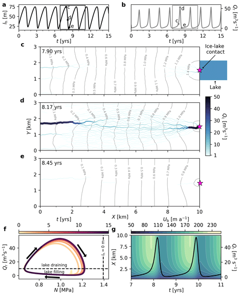
Why does changing the englacial void ratio change the Greenland case’s behavior so much, but not the synthetic case? Why does the synthetic case never surpass flotation pressure, while the Greenland case consistently does? You are making the argument that the long flood durations are partially because GlaDS can’t deal with uplift, but the synthetic case seems to still be showing monthslong flood durations without ever going near flotation pressures (Fig. 2b) – so this argument may not hold. I would also love to see another sensitivity test where you change the englacial void ratio (Fig. 3)
Fig. 5: it would be helpful to show f and g on the same axes (modeled & observed) to understand the difference between them
I like that you tried changing the channel and sheet conductivity. Can you provide some additional comments about some real-world cases where you might see higher or lower sheet or channel conductivity? What kind of bed types or drainage configurations would lead to seeing these conditions in real life?
L394: Why do you think your assumption of a continuous sheet to be more physically plausible than the isolated cavity assumption? Wouldn’t this change from glacier to glacier? Can you try running the jokulhlaup with the lake NOT connected directly to the sheet, and would this affect the results?
L400 ish: Can you comment more on why the response to basal melt is so different with GlaDS and the Kingslake and Ng (2013) result?
Figure 7: why is v_b much larger for the modelled than the observed? Why are observed flood anomalies so much larger than modelled flood anomalies? Later in the discussion you say the model is an underestimate but it seems the other way around, based on model/observation comparison. Can you account for this?
L450: what about the other two subglacial lakes? Although the flowpath passes through anomaly 1, do the model results support the formation of a subglacial lake there?
L476: can you comment more specifically on the limitations of your model setup? What aspects of the model setup could improve your approach? You did a nice job explaining the limitations of GlaDS but would love to hear more about the continuity eqns, boundary conditions, etc that was added to the default GlaDS setup.
Minor comments
L174: Can you provide a citation or justification for initializing phi at 90% of the overburden pressure? Same thing with the initial sheet thickness.
L176: Please specify what you mean by “the other three boundaries”
L227: What do you mean by “vigorous”? I would use a more quantitative phrasing here.
Line 256 – typo in “anisotropic”
Figure 4 – graphically specify high k_c case and low k_c case for additional clarity (rather than just high case, low case)
L405: Since not all readers will be doing a detailed read of the full manuscript, I wonder if this discussion could use the full words rather than the variable names. Otherwise it’s a bit challenging to go back and forth to understand what each variable is.
L437: what happened to the final flood that was not hindcasted by the model? You discuss this later (that your model does not account for glacier thinning which could help trigger an additional jokulhlaup) but could be good to mention either that you will discuss it later or provide some quick explanation here before moving on.
Citation: https://doi.org/10.5194/egusphere-2026-2948-RC2 - AC2: 'Reply on RC2', Adam Jake Hepburn, 01 Sep 2026
Peer review completion
Journal article(s) based on this preprint
Model code and software
pyJokulhlaup A. J. Hepburn https://github.com/The-SLIDE-Project/pyJokulhlaup
Viewed
| HTML | XML | Total | BibTeX | EndNote | |
|---|---|---|---|---|---|
| 232 | 99 | 27 | 358 | 22 | 19 |
- HTML: 232
- PDF: 99
- XML: 27
- Total: 358
- BibTeX: 22
- EndNote: 19
Viewed (geographical distribution)
| Country | # | Views | % |
|---|
| Total: | 0 |
| HTML: | 0 |
| PDF: | 0 |
| XML: | 0 |
- 1

Sammie Buzzard
Andrew J. Sole
Stephen J. Livingstone
Mathieu Morlighem
Elizabeth A. Bagshaw
Caroline Clason
Lisa Craw
Christine Dow
Samuel Doyle
Jonathan Hawkins
Matthew Peacey
Robert Storrar
The requested preprint has a corresponding peer-reviewed final revised paper. You are encouraged to refer to the final revised version.
- Preprint
(5374 KB) - Metadata XML
This is a interesting and well written paper that presents the results of a coupled conduit–sheet model of jökulhlaups based on the subglacial hydrology model GLaDS for both a synthetic glacier and for the Isunnguata Sermia glacier in W-Greenland, which is known for semi-regular jökulhlaups every 2–4 years. The model includes coupling with the flow of the overlying glacier implemented with the ISSM ice-flow model. The model represents a significant advance over earlier models of similar type. The simulated jökulhlaups from Isunnguata Sermia are nevertheless longer in duration (by more than an order of magnitude!) and have too small maximum discharge compared with observations. The authors attribute this failure of the model to its inability to capture large-scale, elastic lifting of the glacier as there is "no physical representation of elastic uplift of ice once water pressure exceeds ice overburden pressure". This makes sense and underlines the need to include this physics in future work on jökulhlaup dynamics. The coupling with ice flow and basal sliding reproduces some features of the observed response of the Isunnguata Sermia glacier to jökulhlaups but the lack of quantitative agreement regarding the magnitude and spatial patterns of anomalies in surface ice velocity shows that jökulhlaup models are still not able to faithfully represent the underlying dynamics in the coupled subglacial hydrology – ice flow problem, but the presented model is, nevertheless, a significant step forward.
Comments:
1. There is a brief model description on p. 5–6 and in Appendix B. This includes explanations of model model parameters and variables that are studied later in the paper. However, the variable l_c (channel sheet width) and M_r (basal melt rate) are not explained although they are part of the sensitivity analysis shown in Figure 3. Consider adding a short description of these parameters/variables.
2. In l. 102/103 you say "As in the model of Kingslake and Ng (2013), we do not account for frictional heating in our solution." If you are just explaining that the model assumes the water to be at the pressure melting point, it would be better to just say that. The assumption that the water is maintained at the pressure melting point means that potential energy is dissipated through friction in the water flow so that frictional "heating" is in fact represented in the model although the water cannot be said to be heated. Perhaps clarify this statement?
3. In Eq. (2), the y-component of the basal sliding velocity (v_b) appears in the numerator but the x-component does not. This seems strange. Consider whether this is as intended. Also, you might briefly explain the difference between the formulation of the Schoof-type sliding law in ISSM and the more well-known original formulation by Schoof.
4. In lines 375–377 you state that "Ice near to the lake accelerates markedly" but in fact the acceleration affects a much larger area. Clarify. You also mention that "Such a velocity pattern has been observed during jökulhlaups at ... Skaftá by Magnússon et al. (2007). The velocity pattern observed by Magnússon affects almost the entire Skaftárjökull outlet glacier, not just an area near the subglacial lake. Clarify this also. You might call this location "Skaftá cauldrons" as Skaftá is the name of the river outside the glacier, whereas the jökulhlaups in question are released from cauldrons in W-Vatnajökull called Skaftá cauldrons.
5. In l. 399 you mention melt rates of 1 m a^{−1} to 5 m a^{−1}. These seem very high. Explain.
6. In l. 437 you explain that "Of these floods, seven are hindcasted by our model (Fig. 5f), closely agreeing with observations in terms of timing and the amplitude of change in l_h." This is impressive but you might explain that this success is mainly a consequence of the fitting of the simulated inflow to the lake with a degree−day model and the capacity of the lake which depends on easily measured quantities and continuity (assuming that the lake will eventually drain at a high stand for more or less any subglacial hydrology model configuration). The success of the impressive fitting to the observed variations in the lake level is only indirectly caused by the coupled subglacial hydrology − ice flow model, which is the main subject of the paper. Explain briefly how the successful fitting to the lake level variation is achieved and that it does not necessarily reflect successful simulations of the subglacial hydrology.
7. Did Flowers et al. (2004) really work with sheet thicknesses exceeding tens of metres (l. 486) (?). This seems excessive. In the 2004 GRL paper, she mentions 7–11 m sheet thickness. If you are referring to this range you should say "sheet thicknesses on the order of ten metres" or something like that. This sheet thickness magnitude refers to Björnsson's (1997) interpretation of observations of the catastrophic 1996 jökulhlaup from Grímsvötn, which you might find worth referencing in this context.
In the following sentence (l. 486−488) you state "Recent repeat satellite observations identified metres of uplift along a jökulhlaup pathway ..." quoting Magnússon et al. (2026). The lifting reported by Magnússon et al. was close 1 m. Please clarify. Maybe say "identified appoximately 1 metre of uplift" or "identified ~1 metre of uplift" about Magnússon's observations.
8. In l. 518-519, you state: "... and recognizing that our model successfully reproduces flood timing across a multidecadal record without tuning to individual events, we view the discrepancies in duration and peak as a tractable modelling challenge rather than a fundamental limitation." The successful reproduction of the flood timing is interesting, but as I mention above does not, in my opinion, have much to do with the coupled subglacial hydrology − ice flow model developed in the paper. It seems to me that in order to reproduce the short flood duration and higher maximum discharge, a substantial improvement in the model is necessary, such as the implementation of large-scale (elastic) lifting of the ice from the bed, as stated in the paper at several places. This would be a fundamental improvement, so the sentence that I quote above is perhaps too optimistic or describes this to lightly, although I hope this problem is indeed "tractable".
Minor and editorial comments: