
the Creative Commons Attribution 4.0 License.
the Creative Commons Attribution 4.0 License.
 | 06 May 2026
Synthesis of the tethered balloon system and other TRACER campaign measurements elucidates aerosol property profiles
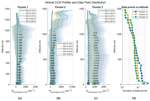
Abstract. Coastal urban environments exhibit strong vertical and horizontal heterogeneity in aerosol properties, complicating process-level understanding of aerosol–cloud interactions. This study analyzes tethered balloon system (TBS) measurements from 149 flights during summer over the greater Houston, Texas, region as part of the DOE Atmospheric Radiation Measurement (ARM) Tracking Aerosol Convection interactions ExpeRiment (TRACER) campaign. We characterize the vertical structure of aerosol number concentrations, size distributions, and inferred cloud condensation nuclei (CCN) concentrations. Air mass history was classified using back-trajectory analysis and k-means clustering into three clusters: (1) marine-influenced, (2) mixed marine and urban emissions, and (3) urban/anthropogenic and long-range transported aerosols. CCN concentrations are estimated from observed size distributions using κ-Köhler theory. The resulting profiles show pronounced vertical variability across clusters, strongly modulated by boundary-layer depth and coastal circulations, leading to substantial variability in the aerosol population available for cloud activation. The marine cluster showed the lowest concentrations, with CCN at 0.8 % supersaturation below 1,000 cm⁻³, while urban and mixed clusters displayed higher concentrations and more complex layering. Profiles influenced by the mixed marine–urban cluster frequently exhibit decoupling between near-surface aerosol and elevated layers, including enhanced accumulation-mode number aloft, consistent with prior TBS-based compositional studies. A September 6–7, 2022 case study demonstrates that mesoscale transport can simultaneously transform both the thermodynamic environment and aerosol population, highlighting the importance of constraining boundary-layer dynamics and airmass origin before attributing cloud changes to aerosol effects in complex coastal environments.
-
Notice on discussion status
The requested preprint has a corresponding peer-reviewed final revised paper. You are encouraged to refer to the final revised version.
-
Preprint
(3570 KB)
-
Supplement
(2398 KB)
-
The requested preprint has a corresponding peer-reviewed final revised paper. You are encouraged to refer to the final revised version.
- Preprint
(3570 KB) - Metadata XML
-
Supplement
(2398 KB) - BibTeX
- EndNote
- Final revised paper


Journal article(s) based on this preprint
Interactive discussion
Status: closed
-
RC1: 'Comment on egusphere-2026-2245', Anonymous Referee #1, 19 Jun 2026
-
AC1: 'Reply on RC1', Fan Mei, 25 Aug 2026
We sincerely thank the reviewer for the constructive comments and suggestions, which have helped us improve the manuscript. We have revised the manuscript accordingly and provide our point-by-point responses below; a version of the manuscript with all changes marked is also included.
-
AC1: 'Reply on RC1', Fan Mei, 25 Aug 2026
-
RC2: 'Comment on egusphere-2026-2245', Anonymous Referee #2, 30 Jun 2026
The paper titled "Synthesis of the tethered balloon system and other TRACER campaign measurements elucidates aerosol property profiles" reports a topic of a great interest concernig the aerosol vertical profiles.
Here below my major and minor comments listed from the abstract till the conclusions of the paper:
Abstract:
- Lines 17: explain DOE (Department of Energy?)
Section 2.1:
- Line 101: "June to September 2022". Please specify why the campaign was planned in summer and if other campaigns are planned in other seasons
- Figure 1 does not report the transects cited at line 113
Section 2.2:
- Inlcude a picture of payload (described in table 1) of the TBS
- Lines 138-139: report briefly even in the present paper the frequency distribution of TBS profiles per hour of day. It is needed for the environmental and meteorological context of TBS soundings
- Lines 145-151: you used stage D of STAC. What about the other stages?
- Lines 166-170: provide here the methodology, equations and parameters used for Lidar f(RH) corrections. Please note that as reported by Martin (2000, DOI: 10.1021/cr990034t), the aerosol can be humid even below the activation relative humidity depending on RH history and efflorescence RH. As you used RH vertical profiles, discuss the limitation of your approach in the context of the scientific literature as above and the lack of temporal trend of RH with height.
- Line 168: "CCN count measurements": as in section 2.3 you estimated it. As the Lines 166-170 are also based on CCN data, discuss the error of f(RH) even considering the fact that CCN are estimated
Section 2.3:
- The size distribution interpolation and log-normal reconstruction is feasible only if the POPS data are corrected with respect to aerosol refractive index, laser properties of POPS and POPS inner geometry. Improve this section with such calculations (Heyder et al., 1979: Optimization of response functions of light scattering instruments for size evaluation of aerosol particles. Appl Opt 1979;18(5):705–11), compare them with the original ones and redo the CCN estimation based on new POPS size distribution interpolation. Consider that POPS can bring undersizing (Guyon et al., 2003: Refractive index of aerosol particles over the Amazon tropical forest during LBA-EUSTACH 1999. J Aerosol Sci 2003;34:883–907). As one of the goal of the present manuscript is related to CCN, its methodology has to be perfect.
- Line 180: please also add as a control the comparison between the fitted size distribution number concentration between 10 and 135 nm obtained as difference between CPC and POPS
- Line 182-184: please discuss the assumption of an homogeneous chemical composition. What about vertical formation of secondary aerosol components. Please discuss this part with respect to scientific literature referred to the context of TBS. Finally, also discuss the limitation of a chemical change with altitude with respect to aerosol refractive index and therefore POPS size correction.
- Line 191: add the densities used for the volumetric average
Section 3.2:
- Figure 4: As Ran et al. (2016, doi:10.5194/acp-16-10441-2016) did, when averaging vertical profiles of aerosol it is necessary to use a normalized height with respect to the PBL calculated from h/PBL_height−1; Please compute again vertical profiles average in Figure 4 to check them and compare with the absolute altitude averaged profiles to ensure consistency within the environental interpretations of the results, for example the assertion that "This suggests that the local-scale thermal structure and boundary-layer depth were not strongly dependent on air-mass origin during the sampled period...". This is what you did in section 3.4 for CCN profiles
- Figure 4: panels c) and d) are inverted, moreover the panel letter is missing within the figure
- Line 288: "subtle"? Suitable?
- Line 314: "new particle formation". With the present apparatus it is impossibile to speculate about it. Please remove the statement.
Section 3.4:
- Results seems interesting, however refer to my comment related to section 2.3 and POPS size distribution correction before interpolation and CCN determination. After the number size distribution correction and new CCN determination results have to be updated. The same happens for section 3.5
- Lines 434-437: you assumed homogeneous chemical composition.... these lines are mostly a matter of speculation, please remove them
- Figure 7 lacks of panel letters
- What about number size distribution change with altitute in respect to CCN? Please add the vertical profiles of mean diameter and geometric standard deviations of the modes interpolated for each cluster and compare them with CCN
Section 3.5:
- Panel labels of Figures 8, 9 and 10 are missing
PLEASE PROVIDE AN ACRONYMS TABLE OR APPENDIX
Citation: https://doi.org/10.5194/egusphere-2026-2245-RC2 - AC2: 'Reply on RC2', Fan Mei, 25 Aug 2026
Peer review completion


Interactive discussion
Status: closed
-
RC1: 'Comment on egusphere-2026-2245', Anonymous Referee #1, 19 Jun 2026
The study by Mei et al. presents tethered balloon measurements complemented by surface-based and remote sensing observations and ancillary calculations conducted during the TRACER campaign, offering a highly valuable contribution to the field. The work builds upon previous research and draws on multi-platform measurements and derived data techniques. The detailed analysis effectively demonstrates the necessity of integrating distinct observation types to gain a more comprehensive understanding of the atmospheric processes involved. In particular, the aerosol concentrations and estimated CCN profiles provide new insights into the vertical distribution of aerosol properties as influenced by air mass origin. The extensive set of tethered balloon profiles enables the identification of distinct clusters and provide compelling statistics spanning the summer through early fall seasons. The case study from September 6–7 further illustrates the complexity of the atmospheric processes at play and reaffirms the critical role of complementary observational approaches in constructing a temporally and spatially coherent narrative. The authors demonstrate a clear awareness of the study's limitations, including the absence of vertical profiles of particle number size distribution and CCN measurements, the restricted temporal scope of the dataset, and the constraints on the tethered balloon's ability to operate above the boundary layer more frequently. Overall, the manuscript is of high scientific quality, is well-structured, and reads clearly. I recommend accepting the paper subject to minor revisions.
Minor comments:
The description of how the back trajectories are obtained might be better suited to the Data & Methodology section (lines 205-214), after which the results can be directly introduced in section 3.1 (from line 215 onward). A similar consideration might apply to the description of the Principal Component Analysis, which could also be relocated to the methods section.
Ground-based Scanning Mobility Particle Sizer, POPS, and CCN counter instruments appear to have been operated during the deployment, though the specific location remain unclear. For this study, it would be valuable to incorporate ground-based particle number size distributions from 10 nm to 3000 nm. Presenting monthly medians alongside 25th–75th percentile ranges would help visualize concentrations for each mode and assess seasonal variations, providing surface-level measurements representative of the tethered balloon deployment periods. A similar figure could be envisioned for CCN, enabling a direct comparison between measured and estimated CCN at the ground. Additionally, markers representing surface measurements should be displayed at the base of the profiles in Figure 4 for each cluster. If data are available, markers corresponding to measured CCN at the surface should also be added into Figure 7.
Can you please clarify how the flights were grouped into cluster in section 3.2? It appears that the air mass origin defining each cluster influenced entire days or extended periods, allowing individual flights to be categorized accordingly. However, as illustrated by the case study on September 6, a vertical profile was influenced by two distinct air masses associated with Custer 1 and 2. In the case of such decoupled air masses, how were the corresponding flights classified? Alternatively, given that decoupled profiles were rarely encountered during the deployment, were they excluded from Figure 4? Including a figure, table, or calendar displaying the tethered balloon flight times alongside their identified clusters would help visualize the temporal distribution of the air masses sampled throughout the deployment period.
Given the estimated CCN concentration is based on particle hygroscopicity, which is influenced by the volume fraction of each chemical species (Section 2.3), were the volume fractions adjusted to reflect the chemical composition observed aloft in the upper part of the profile on September 6 (Figure 9)? If so, did this yield a different κCCN value, and, consequently, distinct estimated CCN concentrations compared to those derived for the lower part of the profile? Alternatively, are changes in estimated CCN seen above 1000 m in Figure 8a solely attributable to variations in aerosol number concentration?
A compelling case is presented in Section 3.5.3 , differentiating between what might have been anticipated from the case study and the conditions that were actually observed by combining aerosols, and thermodynamic variables. The importance of integrating multiple observation types to fully capture such an event is clearly demonstrated. Could you elaborate further on the broader implications of these findings from a climate perspective? What insights does this case study offer within a larger climate context? What does it reveal about our understanding of the climate processes for this region?
Specific comments:
Line 105: “ a co-located microwave radiometer”, which model was used? Is there a publication associated with this instrument?
Line 141: Table 1. Would it be possible to replace the “instruments” column with two separate columns: one listing the name and model of each instrument, and a second one providing the manufacturer’s name? The current column includes some model names but does not consistently identify the manufacturers.
Line 168: For clarification, where were the ground-based SMPS, POPS, and CCN counter located? Were they deployed at La Porte?
Line 183: The calculation of CCN using the κ-Köhler theory assumes a uniform aerosol chemical composition from the surface up through the vertical column. Based on the meteorological profiles obtained from the tethered balloon, were any decoupled layers aloft identified during the campaign beside the case study? If so, do you have any statistics on their frequency of occurrence?
Line 190: Has the uncertainty introduced by the assumption of vertically uniform chemical composition been quantified in previous studies?
Line 236: Could you provide a reference describing the Principal Component Analysis methodology? This would be helpful for readers unfamiliar with this method, allowing them to access further details on the approach and potential examples of its application.
Line 280: Please rename Npops and Ncpc using the corresponding particle size ranges, N135-3000 N>10 in both the text and the figures.
Line 289: Subtle temperature differences are described at the surface between the clusters. Are these differences significant? Could they be explained by the topography and/or the wind direction? If these differences cannot be attributed to air mass origin, presenting the numbers without further context may be misleading to the reader.
Line 300: It seems that DMS has not been introduced before.
Line 316, Figure 4: Could the surface measurements be added at the bottom of the vertical profiles, using a distinct maker or other visual differentiation? It would make it insightful to display the tethered balloon observations and ground-based reference instrument measurements in the same figure. This comment is associated with previous general feedback on displaying surface-based observations.
Line 458: Could you specify the take-off and landing times for the flights on September 6 (and September 7)? Although the flight is represented in Figure 6 between 15:30 and 18:30, a reminder in the text would help the reader follow the discussion more easily.
Line 465: Have you examined 5-day back trajectories for September 6 and 7? Do the longer back trajectories support the assumption of long-range transport for the overlying aerosol layer? Additionally, have you considered visualizing the back trajectories with time on the x-axis, altitude on the y-axis, and an indication of whether the air mass traveled below or above the boundary layer during its transport? Potential supplementary figures presenting these analyses could further reinforce the narrative of the case study.
Line 475, Figure 8: Could the pressure levels in Figure 8c and 8d be converted to altitude? It would facilitate a more direct comparison with Figure 8a.
Line 520: CAPE has not been introduced before.
Technical comments:
Line 62: A period is missing between “and chemical composition” and “Airborne platforms”.
Line 397: When referring to Figures (a)–(c), do you mean Figures 7 and S2? Please clarify and ensure the figure references are correct.
Line 460: a period is missing between “increase with altitude" and "These trends”.
Line 471: Figure S8 is introduced before Figure S4 in the reading order. Please consider renumbering the supplementary figures to follow the sequential order in which they are first cited in the text.
Line 483 and following paragraphs: mb and hPa are used throughout. Please harmonize the units to SI standards by using hPa consistently throughout the manuscript.
Figure S6: The legend appears to be incorrect. Please update it with the appropriate and correct legend.
Citation: https://doi.org/10.5194/egusphere-2026-2245-RC1 -
AC1: 'Reply on RC1', Fan Mei, 25 Aug 2026
We sincerely thank the reviewer for the constructive comments and suggestions, which have helped us improve the manuscript. We have revised the manuscript accordingly and provide our point-by-point responses below; a version of the manuscript with all changes marked is also included.
-
AC1: 'Reply on RC1', Fan Mei, 25 Aug 2026
-
RC2: 'Comment on egusphere-2026-2245', Anonymous Referee #2, 30 Jun 2026
The paper titled "Synthesis of the tethered balloon system and other TRACER campaign measurements elucidates aerosol property profiles" reports a topic of a great interest concernig the aerosol vertical profiles.
Here below my major and minor comments listed from the abstract till the conclusions of the paper:
Abstract:
- Lines 17: explain DOE (Department of Energy?)
Section 2.1:
- Line 101: "June to September 2022". Please specify why the campaign was planned in summer and if other campaigns are planned in other seasons
- Figure 1 does not report the transects cited at line 113
Section 2.2:
- Inlcude a picture of payload (described in table 1) of the TBS
- Lines 138-139: report briefly even in the present paper the frequency distribution of TBS profiles per hour of day. It is needed for the environmental and meteorological context of TBS soundings
- Lines 145-151: you used stage D of STAC. What about the other stages?
- Lines 166-170: provide here the methodology, equations and parameters used for Lidar f(RH) corrections. Please note that as reported by Martin (2000, DOI: 10.1021/cr990034t), the aerosol can be humid even below the activation relative humidity depending on RH history and efflorescence RH. As you used RH vertical profiles, discuss the limitation of your approach in the context of the scientific literature as above and the lack of temporal trend of RH with height.
- Line 168: "CCN count measurements": as in section 2.3 you estimated it. As the Lines 166-170 are also based on CCN data, discuss the error of f(RH) even considering the fact that CCN are estimated
Section 2.3:
- The size distribution interpolation and log-normal reconstruction is feasible only if the POPS data are corrected with respect to aerosol refractive index, laser properties of POPS and POPS inner geometry. Improve this section with such calculations (Heyder et al., 1979: Optimization of response functions of light scattering instruments for size evaluation of aerosol particles. Appl Opt 1979;18(5):705–11), compare them with the original ones and redo the CCN estimation based on new POPS size distribution interpolation. Consider that POPS can bring undersizing (Guyon et al., 2003: Refractive index of aerosol particles over the Amazon tropical forest during LBA-EUSTACH 1999. J Aerosol Sci 2003;34:883–907). As one of the goal of the present manuscript is related to CCN, its methodology has to be perfect.
- Line 180: please also add as a control the comparison between the fitted size distribution number concentration between 10 and 135 nm obtained as difference between CPC and POPS
- Line 182-184: please discuss the assumption of an homogeneous chemical composition. What about vertical formation of secondary aerosol components. Please discuss this part with respect to scientific literature referred to the context of TBS. Finally, also discuss the limitation of a chemical change with altitude with respect to aerosol refractive index and therefore POPS size correction.
- Line 191: add the densities used for the volumetric average
Section 3.2:
- Figure 4: As Ran et al. (2016, doi:10.5194/acp-16-10441-2016) did, when averaging vertical profiles of aerosol it is necessary to use a normalized height with respect to the PBL calculated from h/PBL_height−1; Please compute again vertical profiles average in Figure 4 to check them and compare with the absolute altitude averaged profiles to ensure consistency within the environental interpretations of the results, for example the assertion that "This suggests that the local-scale thermal structure and boundary-layer depth were not strongly dependent on air-mass origin during the sampled period...". This is what you did in section 3.4 for CCN profiles
- Figure 4: panels c) and d) are inverted, moreover the panel letter is missing within the figure
- Line 288: "subtle"? Suitable?
- Line 314: "new particle formation". With the present apparatus it is impossibile to speculate about it. Please remove the statement.
Section 3.4:
- Results seems interesting, however refer to my comment related to section 2.3 and POPS size distribution correction before interpolation and CCN determination. After the number size distribution correction and new CCN determination results have to be updated. The same happens for section 3.5
- Lines 434-437: you assumed homogeneous chemical composition.... these lines are mostly a matter of speculation, please remove them
- Figure 7 lacks of panel letters
- What about number size distribution change with altitute in respect to CCN? Please add the vertical profiles of mean diameter and geometric standard deviations of the modes interpolated for each cluster and compare them with CCN
Section 3.5:
- Panel labels of Figures 8, 9 and 10 are missing
PLEASE PROVIDE AN ACRONYMS TABLE OR APPENDIX
Citation: https://doi.org/10.5194/egusphere-2026-2245-RC2 - AC2: 'Reply on RC2', Fan Mei, 25 Aug 2026
Peer review completion
Journal article(s) based on this preprint
Viewed
| HTML | XML | Total | Supplement | BibTeX | EndNote | |
|---|---|---|---|---|---|---|
| 424 | 277 | 49 | 750 | 49 | 43 | 47 |
- HTML: 424
- PDF: 277
- XML: 49
- Total: 750
- Supplement: 49
- BibTeX: 43
- EndNote: 47
Viewed (geographical distribution)
| Country | # | Views | % |
|---|
| Total: | 0 |
| HTML: | 0 |
| PDF: | 0 |
| XML: | 0 |
- 1

Jian Wang
Israel Silber
Nurun Nahar Lata
Gregory W. Vandergrift
Sarah Brooks
Michael P. Jensen
Damao Zhang
Darielle Dexheimer
Beat Schmid
Zezhen Cheng
Swarup China
The requested preprint has a corresponding peer-reviewed final revised paper. You are encouraged to refer to the final revised version.
- Preprint
(3570 KB) - Metadata XML
-
Supplement
(2398 KB) - BibTeX
- EndNote
- Final revised paper
The study by Mei et al. presents tethered balloon measurements complemented by surface-based and remote sensing observations and ancillary calculations conducted during the TRACER campaign, offering a highly valuable contribution to the field. The work builds upon previous research and draws on multi-platform measurements and derived data techniques. The detailed analysis effectively demonstrates the necessity of integrating distinct observation types to gain a more comprehensive understanding of the atmospheric processes involved. In particular, the aerosol concentrations and estimated CCN profiles provide new insights into the vertical distribution of aerosol properties as influenced by air mass origin. The extensive set of tethered balloon profiles enables the identification of distinct clusters and provide compelling statistics spanning the summer through early fall seasons. The case study from September 6–7 further illustrates the complexity of the atmospheric processes at play and reaffirms the critical role of complementary observational approaches in constructing a temporally and spatially coherent narrative. The authors demonstrate a clear awareness of the study's limitations, including the absence of vertical profiles of particle number size distribution and CCN measurements, the restricted temporal scope of the dataset, and the constraints on the tethered balloon's ability to operate above the boundary layer more frequently. Overall, the manuscript is of high scientific quality, is well-structured, and reads clearly. I recommend accepting the paper subject to minor revisions.
Minor comments:
The description of how the back trajectories are obtained might be better suited to the Data & Methodology section (lines 205-214), after which the results can be directly introduced in section 3.1 (from line 215 onward). A similar consideration might apply to the description of the Principal Component Analysis, which could also be relocated to the methods section.
Ground-based Scanning Mobility Particle Sizer, POPS, and CCN counter instruments appear to have been operated during the deployment, though the specific location remain unclear. For this study, it would be valuable to incorporate ground-based particle number size distributions from 10 nm to 3000 nm. Presenting monthly medians alongside 25th–75th percentile ranges would help visualize concentrations for each mode and assess seasonal variations, providing surface-level measurements representative of the tethered balloon deployment periods. A similar figure could be envisioned for CCN, enabling a direct comparison between measured and estimated CCN at the ground. Additionally, markers representing surface measurements should be displayed at the base of the profiles in Figure 4 for each cluster. If data are available, markers corresponding to measured CCN at the surface should also be added into Figure 7.
Can you please clarify how the flights were grouped into cluster in section 3.2? It appears that the air mass origin defining each cluster influenced entire days or extended periods, allowing individual flights to be categorized accordingly. However, as illustrated by the case study on September 6, a vertical profile was influenced by two distinct air masses associated with Custer 1 and 2. In the case of such decoupled air masses, how were the corresponding flights classified? Alternatively, given that decoupled profiles were rarely encountered during the deployment, were they excluded from Figure 4? Including a figure, table, or calendar displaying the tethered balloon flight times alongside their identified clusters would help visualize the temporal distribution of the air masses sampled throughout the deployment period.
Given the estimated CCN concentration is based on particle hygroscopicity, which is influenced by the volume fraction of each chemical species (Section 2.3), were the volume fractions adjusted to reflect the chemical composition observed aloft in the upper part of the profile on September 6 (Figure 9)? If so, did this yield a different κCCN value, and, consequently, distinct estimated CCN concentrations compared to those derived for the lower part of the profile? Alternatively, are changes in estimated CCN seen above 1000 m in Figure 8a solely attributable to variations in aerosol number concentration?
A compelling case is presented in Section 3.5.3 , differentiating between what might have been anticipated from the case study and the conditions that were actually observed by combining aerosols, and thermodynamic variables. The importance of integrating multiple observation types to fully capture such an event is clearly demonstrated. Could you elaborate further on the broader implications of these findings from a climate perspective? What insights does this case study offer within a larger climate context? What does it reveal about our understanding of the climate processes for this region?
Specific comments:
Line 105: “ a co-located microwave radiometer”, which model was used? Is there a publication associated with this instrument?
Line 141: Table 1. Would it be possible to replace the “instruments” column with two separate columns: one listing the name and model of each instrument, and a second one providing the manufacturer’s name? The current column includes some model names but does not consistently identify the manufacturers.
Line 168: For clarification, where were the ground-based SMPS, POPS, and CCN counter located? Were they deployed at La Porte?
Line 183: The calculation of CCN using the κ-Köhler theory assumes a uniform aerosol chemical composition from the surface up through the vertical column. Based on the meteorological profiles obtained from the tethered balloon, were any decoupled layers aloft identified during the campaign beside the case study? If so, do you have any statistics on their frequency of occurrence?
Line 190: Has the uncertainty introduced by the assumption of vertically uniform chemical composition been quantified in previous studies?
Line 236: Could you provide a reference describing the Principal Component Analysis methodology? This would be helpful for readers unfamiliar with this method, allowing them to access further details on the approach and potential examples of its application.
Line 280: Please rename Npops and Ncpc using the corresponding particle size ranges, N135-3000 N>10 in both the text and the figures.
Line 289: Subtle temperature differences are described at the surface between the clusters. Are these differences significant? Could they be explained by the topography and/or the wind direction? If these differences cannot be attributed to air mass origin, presenting the numbers without further context may be misleading to the reader.
Line 300: It seems that DMS has not been introduced before.
Line 316, Figure 4: Could the surface measurements be added at the bottom of the vertical profiles, using a distinct maker or other visual differentiation? It would make it insightful to display the tethered balloon observations and ground-based reference instrument measurements in the same figure. This comment is associated with previous general feedback on displaying surface-based observations.
Line 458: Could you specify the take-off and landing times for the flights on September 6 (and September 7)? Although the flight is represented in Figure 6 between 15:30 and 18:30, a reminder in the text would help the reader follow the discussion more easily.
Line 465: Have you examined 5-day back trajectories for September 6 and 7? Do the longer back trajectories support the assumption of long-range transport for the overlying aerosol layer? Additionally, have you considered visualizing the back trajectories with time on the x-axis, altitude on the y-axis, and an indication of whether the air mass traveled below or above the boundary layer during its transport? Potential supplementary figures presenting these analyses could further reinforce the narrative of the case study.
Line 475, Figure 8: Could the pressure levels in Figure 8c and 8d be converted to altitude? It would facilitate a more direct comparison with Figure 8a.
Line 520: CAPE has not been introduced before.
Technical comments:
Line 62: A period is missing between “and chemical composition” and “Airborne platforms”.
Line 397: When referring to Figures (a)–(c), do you mean Figures 7 and S2? Please clarify and ensure the figure references are correct.
Line 460: a period is missing between “increase with altitude" and "These trends”.
Line 471: Figure S8 is introduced before Figure S4 in the reading order. Please consider renumbering the supplementary figures to follow the sequential order in which they are first cited in the text.
Line 483 and following paragraphs: mb and hPa are used throughout. Please harmonize the units to SI standards by using hPa consistently throughout the manuscript.
Figure S6: The legend appears to be incorrect. Please update it with the appropriate and correct legend.