
the Creative Commons Attribution 4.0 License.
the Creative Commons Attribution 4.0 License.
 | 24 Oct 2025
Advective, adiabatic and diabatic contributions to heat extremes simulated with the Community Earth System Model version 2
Abstract. Do heat extremes in climate model simulations form for the right physical reasons? Addressing this question is essential to further our confidence in heat extreme projections, to pinpoint regionally varying model biases, and to enable model improvements regarding heat extremes. Here, we perform a detailed process-based evaluation of CMIP6-type simulations with the Community Earth System Model version 2 (CESM2) regarding heat extremes and employ a Lagrangian approach to quantify advective, adiabatic, and diabatic contributions to near-surface temperature anomalies (T′) during heat extremes. Heat extremes are identified at each grid point and year as the day with the largest daily mean two-meter temperature (hereafter termed TX1day events).
Comparison of CESM2 results with results of an analogous analysis in ERA5 reanalyses for the time period 1980–2020 reveals that, qualitatively and considering continental-scale variations, near-surface T′ during TX1day events in CESM2 form in a physically similar way as in ERA5: Advective contributions dominate in storm track regions, diabatic contributions dominate over tropical and subtropical land regions, and adiabatic warming contributes significantly to heat extremes over subtropical oceans and extratropical land regions. However, quantitatively and at regional scales, there are considerable differences: CESM2 overestimates the magnitude of near-surface T′ during TX1day events in numerous regions (in the global average the TX1day T′ magnitudes are 3.70 K and 3.21 K in CESM2 and ERA5, respectively). These differences are related to larger advective contributions to TX1day events in CESM2 compared to ERA5. That is, biases in the magnitude of simulated TX1day events appear to be related to circulation differences associated with TX1day events in CESM2 as opposed to ERA5. Furthermore, over land, CESM2 systematically overestimates the diabatic contribution to near-surface T′ during TX1day events (4.61 K in CESM2 vs. 2.48 K in ERA5), and underestimates the adiabatic contribution (1.69 K in CESM2 vs. 3.45 K in ERA5). Biases in these contributions to TX1day T′ are much larger than the biases in the TX1day T′ magnitude, and, consequently, the magnitude of CESM2 TX1day events is often “right for the partly wrong physical reasons”. Composite analyses for TX1day events in selected regions suggest that biases in the land-atmosphere coupling, in particular an erroneous partitioning between sensible and latent heat fluxes, is partly responsible for the overestimation of diabatic contributions in CESM2.
We argue that such a detailed quantitative understanding of the differences in the physical processes behind simulated and observed heat extremes is highly relevant for assessing and improving the robustness of heat extreme projections. Our results thus call for analogous investigations with other state-of-the-art models.
Competing interests: At least one of the (co-)authors is a member of the editorial board of Weather and Climate Dynamics.
Publisher's note: Copernicus Publications remains neutral with regard to jurisdictional claims made in the text, published maps, institutional affiliations, or any other geographical representation in this paper. While Copernicus Publications makes every effort to include appropriate place names, the final responsibility lies with the authors. Views expressed in the text are those of the authors and do not necessarily reflect the views of the publisher.-
Notice on discussion status
The requested preprint has a corresponding peer-reviewed final revised paper. You are encouraged to refer to the final revised version.
-
Preprint
(15695 KB)
-
The requested preprint has a corresponding peer-reviewed final revised paper. You are encouraged to refer to the final revised version.
- Preprint
(15695 KB) - Metadata XML
- BibTeX
- EndNote
- Final revised paper


Journal article(s) based on this preprint
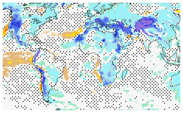
for the partly wrong physical reasons.
Interactive discussion
Status: closed
- RC1: 'Comment on egusphere-2025-5146', Anonymous Referee #1, 06 Dec 2025
-
RC2: 'Comment on egusphere-2025-5146', Osamu Miyawaki, 11 Dec 2025
This manuscript investigates the causes of the difference in the hottest day of the year in ERA5 and CESM2 using Lagrangian backward trajectories. CESM2 generally overestimates the magnitude of the hottest day. This bias is largely associated with the advection term. Advection is further decomposed into a mean state temperature bias and circulation bias, of which the latter dominates the full advection bias. Even in regions where the ERA5 and CESM2 hottest days are similar, there are compensating errors between the adiabatic and diabatic terms, suggesting that in those regions CESM2 gets the right result for the wrong reason.
Quantifying and understanding model biases is important, especially when the model gets the right result for the wrong reasons. I think this manuscript has the potential to be a valuable contribution to quantifying model biases of heat extremes. My main concern is the usefulness of Eq. 1 for understanding heat extremes. Specifically, why is the climatological temperature field used to quantify the advection and adiabatic terms? The intuitive picture I have of advection during an extreme event is the circulation acting on the anomalous temperature field at the time the extreme event, not the climatology. This perspective was also raised by Mayer and Wirth (2025) and Mayer (2025), the latter showing that the Eq. 1 decomposition for the seasonal mean leads to similar results as extremes. This suggests that the differences in the decomposed terms in ERA5 and CESM2 presented here may be dominated by biases in the climatology rather than anomalies therefrom during the extremes. Can the authors better justify using Eq. 1 (as opposed to decomposing based on the anomalous fields as in Mayer) and include in the discussion the advantages and disadvantages of each perspective?
In addition I echo the concerns raised by reviewer 1, especially regarding the inconsistent methods used for ERA5 and CESM2 analyses and the lack of statistical significance. There are several differences between the ERA5 and CESM2 analysis method that may be individually small but is unclear how large they add up to collectively. For example line 533 suggests the modified definition of t_g only has a marginal effect but how much exactly? The most convincing way to resolve these issues is to make the ERA5 and CESM2 analysis like-for-like.
Specific comments:
Line 163: I suggest removing “original” here because the original resolution is 0.25, not 0.5 deg.
Line 190: Fig. 2 -> Fig. 2c
Line 392 and Fig. 10/11b: Oklahoma is too large of an area to describe the location compared to the other regions which seem to be more precise (e.g., city). Also the red star looks farther north than where Oklahoma is.
Line 485: This should specify the vertical resolution used for the Lagranto analysis is not a major reason. It’s not clear whether the native vertical resolution of the dynamical core is important.
References:
Mayer, A., & Wirth, V. (2025). Two different perspectives on heatwaves within the Lagrangian framework. Weather and Climate Dynamics, 6(1), 131-150.
Mayer, A. (2025). A New Global Lagrangian Analysis of Near‐Surface Temperature Extremes. Geophysical Research Letters, 52(19).
Citation: https://doi.org/10.5194/egusphere-2025-5146-RC2 -
AC1: 'Final Author Comment on egusphere-2025-5146', Heini Wernli, 11 Feb 2026
The comment was uploaded in the form of a supplement: https://egusphere.copernicus.org/preprints/2025/egusphere-2025-5146/egusphere-2025-5146-AC1-supplement.pdf
-
EC1: 'Reply on AC1', Ambrogio Volonté, 11 Feb 2026
Dear Authors,
Many thanks for your comprehensive and detailed final response. I note the disagreement between author and reviewers on several of the key reviewers' comments. While in my view those comments are sensible and worth considering, your position is not a plain refusal to adapt your manuscript. Rather, your responses detail the technical constraints and the science aims of this manuscript in a way that was probably not as evident in the original submission. Therefore, I am happy to recommend that you prepare and submit a revised version of this manuscript. I am sure that doing so by addressing the reviewers' comments in the ways detailed in your response will significantly improve your manuscript.
Best wishes
Ambrogio
Citation: https://doi.org/10.5194/egusphere-2025-5146-EC1
-
EC1: 'Reply on AC1', Ambrogio Volonté, 11 Feb 2026
Peer review completion


Interactive discussion
Status: closed
-
RC1: 'Comment on egusphere-2025-5146', Anonymous Referee #1, 06 Dec 2025
Summary
The study by Rothlisberger et al. is a unique approach to understanding potential biases in the Community Earth System Model (CESM) relative to ERA5 reanalysis for the representation of heat extremes. The methodology is interesting and the findings are so far a compelling argument for more in-depth process-level analysis of model behavior. That said, I believe the study requires major revisions to be accepted. The largest potential bias in the study is the use of different horizontal, vertical, and temporal resolutions for the bulk of the comparison between CESM2 and ERA5. The authors partially address this by a handful of sensitivity experiments with re-gridded ERA5, but the results are somewhat different across those case studies which calls into question the paper’s main findings. In a similar vein, there is no apparent significant testing to determine if the differences between these two model-based products is significant, so it remains difficult to determine if the signals shown here are real. I think this work has the potential to be truly impactful in the field, so certainly recommend that the authors pursue additional analysis as outlined in the specific comments below for this study.
Specific Comments
- Definition of heat extremes – is the hottest day each year truly representative of heat extremes in the model? One could imagine that more important are prolonged (3-5 day) events, and/or those that pass a specific threshold (95th percentile per gridcell over time, e.g.)
- Line 6: “largest daily mean two-meter temperature” – I would specify again here that it’s the largest daily mean anomalous 2 m temperature. Though reading further in the methods, I’m confused since the definition is based on absolute temperature but the values listed in the abstract are anomalies… Why not base the identification of events based on anomalies as well, for consistency?
- Line 42: Very minor, but suggest removing “literally” – unless this is in reference to thermometers actually shattering! In which case, perfect use of the word
- Section 2.1: Although it is useful to note that the setup is the same as used for the CESM2-LE, additional details would make interpreting this paper’s results easier. What horizontal resolution is the model run at? Is this a fully coupled simulation (with ocean actively feeding back with the atmosphere), or AMIP-style?
- Section 2.2: If CESM2 is presumably run at 1 degree resolution, why keep ERA5 data at half degree instead of matching the spatial resolution in CESM2? Similar for the temporal resolution, why not use 6-hourly to match CESM2? I realize the ERA5 analysis was already published, but consistency here would be incredibly beneficial for supporting the findings!
- I see this is noted in Section 2.3; suggest moving up mention of the interpolation.
- Line 124: I don’t know if everyone’s familiar with LAGRANTO 2.0 (I am admittedly not!); it would be worth adding a few sentences to explain how this tool works.
- Line 157: I doubt this will change results much, but again I’d suggest keeping the analysis of ERA5 and CESM2 identical whenever possible; in that case. T_CESM2’s average for 1980-1983 should also stem from 1979-1987 instead of extending back to 1976.
- Figure 2: Some the differences are quite small, as noted in the text around negative delta T’ in 2a, for example. Adding a significance test to determine if the difference is statistically real would strengthen this analysis considerably.
- Figure 3: Suggest removing the difference from the bar charts in (a) and (b); it’s somewhat distracting to consider separately. Also suggest adding an x label to 3c for clarity
- Figure 3c and discussion in the text: Could the legend be moved so as to show the purple line at high deciles? It looks like there’s an interesting change in the bias trend from the 9th to 10th decile that could be worth mentioning. Does this show up if different binning is used? Does it indicate something unique physically about these regions?
- Figure 6: For consistency with other 2-column figures, suggest swapping columns so that the right stays ERA5 and the left stays CESM2.
- Section 3.4.1: Strongly suggest that any comparison between products be done at the same grid to begin with. The 0.5 degree used here is already not really the “native” grid of ERA5 (should be 0.25).
- Table 1: As in other figures, statistical significance would be really helpful here; the values of adiabatic/diabatic T’ seem really large when moving from 0.5 to 1 degree resolution, but is it significant?
- Fig 10: Minor point, but since red shading is used it’s somewhat hard to see the red star indicating the point of interest. Maybe add an outline to the marker for enhanced visibility? Or a different color?
- Fig 10 & 11: I wonder if it would be more straightforward to combine SH and LH fluxes into evaporative fraction or Bowen Ratio; it would be a bit easier to see the differences if it were just one figure/field.
- In general, I’m not sure how much the case studies in Figures 10/11 help illustrate the point, given that as stated in line 403, “the degree to which these case study results can be generalized needs to be evaluated further.” More analysis is needed to identify where/when the flux imbalances are key for heat extremes for this section to be impactful in the current study.
- Lines 426-427: “However, such effects would likely also depend on the (observed and simulated) base state regarding soil moisture, as further drying in already too dry regions may be underestimated in simulations.” – add citations and/or figure refs.
- Lines 434-436: “While the magnitude of TX1day events is modest in these regions, these biases are still worrying, as they point to a rather different physical mechanism leading to TX1day events in CESM2 compared to ERA5 in these regions.” – how important are heat extremes of 1 day length over ocean regions though? While interesting that there are differences, I would imagine that ocean heat events are more impactful for SST, as organisms under the surface are impacted vs 2m temperature.
- Lines 440-441: “Furthermore, we speculate that mesoscale phenomena such as cold pools, which are known to affect temperature variability over subtropical oceans (e.g., Vogel et al., 2021) are resolved even more poorly in CESM2 compared to ERA5.” – This is a tough speculation to support based on the evidence so far presented. Suggest removing or strengthening the analysis to support this notion.
- Lines 445-449: Given the suggestion of how to strengthen the results here seems relatively clear, is there a reason that this analysis is not undertaken as part of this study? Is the data readily available in the CESM2 experiments?
- In general, the inclusion of multiple ensemble members for CESM2 is a positive feature of the study, but there’s rarely mention of spread across ensemble members, statistical significance relative to ERA5, etc.
- Related to the differences in resolution between ERA5 and CESM2, how much of the difference in P (pressure difference of parcel trajectories) is due to the higher vertical resolution in ERA5 compared to CESM2? I would assume that this is a huge factor given the comparatively low resolution in CESM2…
- Section 4.3: In general, this section is repetitive with the previous two in Section 4. Suggest merging any relevant points and condensing accordingly.
- Data and code availability: “CESM2 data and code underlying this work are available from the first author upon request.” This arguably falls short of the current standard for open and reproducible scientist. I suggest archiving all necessary code/data for reproducibility of these results via GitHub, Zenodo, etc.
Citation: https://doi.org/10.5194/egusphere-2025-5146-RC1 -
RC2: 'Comment on egusphere-2025-5146', Osamu Miyawaki, 11 Dec 2025
This manuscript investigates the causes of the difference in the hottest day of the year in ERA5 and CESM2 using Lagrangian backward trajectories. CESM2 generally overestimates the magnitude of the hottest day. This bias is largely associated with the advection term. Advection is further decomposed into a mean state temperature bias and circulation bias, of which the latter dominates the full advection bias. Even in regions where the ERA5 and CESM2 hottest days are similar, there are compensating errors between the adiabatic and diabatic terms, suggesting that in those regions CESM2 gets the right result for the wrong reason.
Quantifying and understanding model biases is important, especially when the model gets the right result for the wrong reasons. I think this manuscript has the potential to be a valuable contribution to quantifying model biases of heat extremes. My main concern is the usefulness of Eq. 1 for understanding heat extremes. Specifically, why is the climatological temperature field used to quantify the advection and adiabatic terms? The intuitive picture I have of advection during an extreme event is the circulation acting on the anomalous temperature field at the time the extreme event, not the climatology. This perspective was also raised by Mayer and Wirth (2025) and Mayer (2025), the latter showing that the Eq. 1 decomposition for the seasonal mean leads to similar results as extremes. This suggests that the differences in the decomposed terms in ERA5 and CESM2 presented here may be dominated by biases in the climatology rather than anomalies therefrom during the extremes. Can the authors better justify using Eq. 1 (as opposed to decomposing based on the anomalous fields as in Mayer) and include in the discussion the advantages and disadvantages of each perspective?
In addition I echo the concerns raised by reviewer 1, especially regarding the inconsistent methods used for ERA5 and CESM2 analyses and the lack of statistical significance. There are several differences between the ERA5 and CESM2 analysis method that may be individually small but is unclear how large they add up to collectively. For example line 533 suggests the modified definition of t_g only has a marginal effect but how much exactly? The most convincing way to resolve these issues is to make the ERA5 and CESM2 analysis like-for-like.
Specific comments:
Line 163: I suggest removing “original” here because the original resolution is 0.25, not 0.5 deg.
Line 190: Fig. 2 -> Fig. 2c
Line 392 and Fig. 10/11b: Oklahoma is too large of an area to describe the location compared to the other regions which seem to be more precise (e.g., city). Also the red star looks farther north than where Oklahoma is.
Line 485: This should specify the vertical resolution used for the Lagranto analysis is not a major reason. It’s not clear whether the native vertical resolution of the dynamical core is important.
References:
Mayer, A., & Wirth, V. (2025). Two different perspectives on heatwaves within the Lagrangian framework. Weather and Climate Dynamics, 6(1), 131-150.
Mayer, A. (2025). A New Global Lagrangian Analysis of Near‐Surface Temperature Extremes. Geophysical Research Letters, 52(19).
Citation: https://doi.org/10.5194/egusphere-2025-5146-RC2 -
AC1: 'Final Author Comment on egusphere-2025-5146', Heini Wernli, 11 Feb 2026
The comment was uploaded in the form of a supplement: https://egusphere.copernicus.org/preprints/2025/egusphere-2025-5146/egusphere-2025-5146-AC1-supplement.pdf
-
EC1: 'Reply on AC1', Ambrogio Volonté, 11 Feb 2026
Dear Authors,
Many thanks for your comprehensive and detailed final response. I note the disagreement between author and reviewers on several of the key reviewers' comments. While in my view those comments are sensible and worth considering, your position is not a plain refusal to adapt your manuscript. Rather, your responses detail the technical constraints and the science aims of this manuscript in a way that was probably not as evident in the original submission. Therefore, I am happy to recommend that you prepare and submit a revised version of this manuscript. I am sure that doing so by addressing the reviewers' comments in the ways detailed in your response will significantly improve your manuscript.
Best wishes
Ambrogio
Citation: https://doi.org/10.5194/egusphere-2025-5146-EC1
-
EC1: 'Reply on AC1', Ambrogio Volonté, 11 Feb 2026
Peer review completion
Journal article(s) based on this preprint
for the partly wrong physical reasons.
Viewed
| HTML | XML | Total | BibTeX | EndNote | |
|---|---|---|---|---|---|
| 2,138 | 952 | 259 | 3,349 | 163 | 173 |
- HTML: 2,138
- PDF: 952
- XML: 259
- Total: 3,349
- BibTeX: 163
- EndNote: 173
Viewed (geographical distribution)
| Country | # | Views | % |
|---|
| Total: | 0 |
| HTML: | 0 |
| PDF: | 0 |
| XML: | 0 |
- 1
Cited


2 citations as recorded by crossref.
- A tale of two hot spells: dominant circulation patterns favouring persistent high temperatures in western Europe D. Pappert & O. Martius https://doi.org/10.1088/1748-9326/ae7f34
- Physical processes leading to extreme day-to-day temperature change – Part 2: Future climate change K. Hamal & S. Pfahl https://doi.org/10.5194/wcd-7-1009-2026
Matthias Röthlisberger
Michael Sprenger
Urs Beyerle
Erich M. Fischer

The requested preprint has a corresponding peer-reviewed final revised paper. You are encouraged to refer to the final revised version.
- Preprint
(15695 KB) - Metadata XML
Summary
The study by Rothlisberger et al. is a unique approach to understanding potential biases in the Community Earth System Model (CESM) relative to ERA5 reanalysis for the representation of heat extremes. The methodology is interesting and the findings are so far a compelling argument for more in-depth process-level analysis of model behavior. That said, I believe the study requires major revisions to be accepted. The largest potential bias in the study is the use of different horizontal, vertical, and temporal resolutions for the bulk of the comparison between CESM2 and ERA5. The authors partially address this by a handful of sensitivity experiments with re-gridded ERA5, but the results are somewhat different across those case studies which calls into question the paper’s main findings. In a similar vein, there is no apparent significant testing to determine if the differences between these two model-based products is significant, so it remains difficult to determine if the signals shown here are real. I think this work has the potential to be truly impactful in the field, so certainly recommend that the authors pursue additional analysis as outlined in the specific comments below for this study.
Specific Comments