
the Creative Commons Attribution 4.0 License.
the Creative Commons Attribution 4.0 License.
 | 24 Feb 2026
Data-Driven Enhancement of Ocean Surface Forcing for Accurate Floating Debris Transport Modelling in the East/Japan Sea
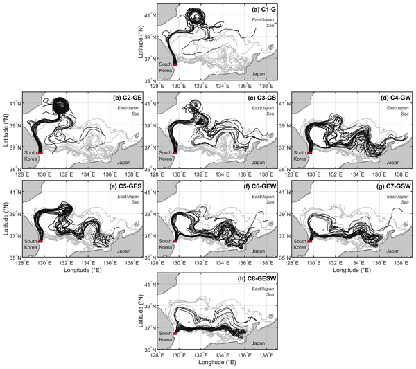
Abstract. The accumulation of floating debris is a growing concern in marginal seas. This study presents the largest surface drifter experiment conducted to date in the East/Japan Sea, utilizing 33 GPS-tracked drifters to calibrate particle tracking models. Deployed off the Korean coast in late fall 2021, the drifters revealed a clear transport conduit to the Japanese coastline, with beaching occurring after an average of 37 to 50 days. We systematically evaluated model performance driven by combinations of geostrophic currents, Ekman currents, Stokes drift, and windage using MAE and NCLS metrics. The results indicate that near-surface debris is best modelled by combining geostrophic currents, Stokes drift, and windage, whereas deeper debris (2-m depth) requires the additional inclusion of Ekman currents. These optimized forcing combinations were found to outperform global circulation models such as HYCOM and CMEMS. Furthermore, seasonal experiments revealed that strong winter winds accelerate eastward transport and beaching along the Japanese coast, while weaker summer winds allow mesoscale eddies to broaden dispersion zones across both Korean and Japanese coastlines. Validated by this extensive dataset, these findings enable more accurate tracking of floating debris in similar basins.
-
Notice on discussion status
The requested preprint has a corresponding peer-reviewed final revised paper. You are encouraged to refer to the final revised version.
-
Preprint
(3572 KB)
-
The requested preprint has a corresponding peer-reviewed final revised paper. You are encouraged to refer to the final revised version.
- Preprint
(3572 KB) - Metadata XML
- BibTeX
- EndNote
- Final revised paper


Journal article(s) based on this preprint
Interactive discussion
Status: closed
-
RC1: 'Comment on egusphere-2026-943', Anonymous Referee #1, 13 Apr 2026
-
AC1: 'Response to RC1', Hong Tran, 18 Jun 2026
We would like to thank the reviewer for the positive and constructive feedback on our manuscript. The revisions made in response to the reviewer's comments have significantly improved the quality and clarity of the manuscript.
For ease of reference:
- Reviewer comments are shown in black text.
- Our responses are provided in red text.
- Revisions and additions made to the manuscript are also highlighted in red.
Kind regards,
Hong Tran Thi My
on behalf of all co-authors
-
AC1: 'Response to RC1', Hong Tran, 18 Jun 2026
-
RC2: 'Comment on egusphere-2026-943', Anonymous Referee #2, 16 Apr 2026
The manuscript investigates the role played by various data derived surface forcings in a Particle Tracking Model (PTM). The results are potentially interesting, but the paper needs major revision before publication. The main issues are indicated below, followed by more specific points.
Main Issues
1) The paper deals with a specific PTM, aimed at reproducing particles moving at the ocean surface and at 2 m depth. While this is a perfectly valid approach, I think the authors should clarify that this is not directly applicable to the transport of macro or micro plastic. Indeed, specific terms should be added to the PTM to simulate the behaviour of plastic debris, depending on their size and characteristics. Such processes include fragmentation, buoyancy changes due to colonization, aggregation and several others. The authors should explain this point up front in the Introduction and Conclusions, i.e. that they focus only on the fluid dynamical part of plastic transport, while for actual applications a number of other processes should included.
2) I am worried about the drifters used in the experiment. No details on drifter testing is provided in Section 2.1, and it is well known that drifters with different properties can move very differently, especially in the very upper part of the ocean. In particular, windage and Stokes drift can be very sensitive to the surface expression. It is important that the authors provide information on the fluid dynamical properties of drifter motion, either using lab experiments or at least quantitatively comparing their motion with that of other drifters with tested properties (such as for instance CODE or CARTHE for the 2m case).
3) The explanation of the datasets and schemes used in the analysis (Section 2.2-2.3) is incomplete and not very clear.
Please explain further the characteristic of the SEALEVEL product, in particular from which satellite observations is obtained and what is the expected physical resolution (aside from the nominal one).
The Ekman layer depth does not seem to have the correct units
The discussion on how windage is computed should be introduced for consistency in Section 2.2 (before eq 5). How are the two r parameter values used in the paper (0.01.5, 0.005) obtained? The authors mention a quite extensive range from the literature; how did they select the two values and did they do some sensitivity tests?
How is the Smagorinsky diffusion coefficient computed? from the geostrophic velocity?
4) The authors mention (line 169 pg 6) that in order to evaluate the PTM versus drifter motion they compute one numerical particle for each drifter initial location. They should clarify whether they actually use an ensemble of particles obtained varying the gaussian random number. Using only one particle, corresponding to a single random realization, would not make sense, and they should repeat the tests using an appropriate ensemble
5) How is the 'cluster' used in section 2.5 to compute relative dispersion defined? Is it given by the total set of drifters released, i.e. using six distinct deployment locations as a single point? Or is it an average of the six individual clusters? The behaviour at initial times seems strange to me
6) The authors state that there is a Hyperbolic Point in the geostrophic velocity, causing the observed bifurcation. I think they should be more precise in their definition; they should look at the FSLE structure from the geostrophic velocity field to verify whether or not the bifurcation is indeed a HP.
7) Also, the reason why the data driven combination outperform the one based on model velocity (Section 4) seems to be that the velocity bifurcation is not present in the model outputs. I find this strange, since the models should assimilate surface height and therefore induce a similar geostrophic velocity with respect to the altimetry products. Can the authors explain this point? And possibly compare the model velocities with the geostrophic one?
8) Results from Ekman and windage (Section 3) are likely to strongly depend on parameterization and parameter values that are very difficult to evaluate. Did they do any sensitivity test? How robust are their conclusions?
9) I cannot see Tab 1-2 in the text
More specific points
1) The definition of PTM should be better clarified when introduced in pg 2. There is a great variety of particle models; often they are based on Eulerian velocity from models outputs, and various types of stochastic terms are considered. In some cases stochastic terms are actually not used at all, if the velocity is assumed to be known with sufficient accuracy, for instance with high resolution models or HF Radars. I think the authors should clarify first of all that they do not include plastic behaviour (see point 1)), and that they use a simple random walk model (eq 4), and focus on Eulerian velocities based on various data sets, each capturing a specific transport processes (geostrophic, Ekman, windage, Stokes drift). Only as a second step they also test model results.
2) Figures should be improved. In Fig.1 it would be useful to have an insert that locates the geographic area. Also, the names of the various lands should be indicated in all the figures, and consistency should be maintained between Fig.1, 2,5, 6 (in terms of area, schematic, data sources, coordinates, names etc..) Also, the arrows in Fig.1b,c are not well visible.
3) Please check for typos. Some examples are:
line 75, (pg 3,) TO validate
line 101(pg 4) THE drifters (instead of these).
title of Section 3 (line 208, pg 8)
Citation: https://doi.org/10.5194/egusphere-2026-943-RC2 -
AC2: 'Response to RC2', Hong Tran, 18 Jun 2026
We would like to thank the reviewer for the positive and constructive feedback on our manuscript. The revisions made in response to the reviewer's comments have significantly improved the quality and clarity of the manuscript.
For ease of reference:
- Reviewer comments are shown in black text.
- Our responses are provided in red text.
- Revisions and additions made to the manuscript are also highlighted in red.
Kind regards,
Hong Tran Thi My
on behalf of all co-authors
-
AC2: 'Response to RC2', Hong Tran, 18 Jun 2026
Peer review completion


Interactive discussion
Status: closed
-
RC1: 'Comment on egusphere-2026-943', Anonymous Referee #1, 13 Apr 2026
This paper discusses simulations and dispersion characteristics of a set of ocean drifters deployed in the East/Japan Sea in 2021.
Whereas the drifter dataset is interesting and deserves publication and thorough analysis, the manuscript has some weaknesses as discussed below. I thus recommend a major revision before eventual publication.
Some general / overall comments:
- A basic trajectory model is described, and used to simulate the trajectories of both surface and drogued drifters with a geostrophic current field + permutations of ekman, Stokes and windage. The analysis is fairly lengthy, just to conclude with what is well known and should be expected: for the surface drifters, all components should be used, whereas for the drifters with drogue at 2m depth, direct wind drag should not be included. As this is all expected, one can question the relevance of all the different combinations used, e.g. using geostrophic current only. It still has some value to confirm what is known, but it could be made much more compact.
- What is more of a question, is the calculation of the windage (wind drift factor) which is a critical component. This is calculated as 1.5% and 0.5% for surface and drogued drifters respectively, but without much details of the exact computation. In any case, this important coefficient will be associated with uncertainty, and it might be more relevant to vary (or even tune) this coefficient, than some of the above mentioned variants which are expected to be not good.
- The Stokes drift is calculated directly from a wave model, and apparently given by Eq 1, but this equation is missing the left side, presumably being the Stokes drift itself. Despite only about 10% of the drifter sticking out of water (~3 of 30 cm), Stokes drift is evaluated at z=0 (surface) and 1.5m (“weighted mean” of surface and drogue at 2m). For the undrogued drifter, a depth of ~15 cm should be more relevant. Difference might not be huge, but (along with uncertain/postulated wind drift factor) might be enough to give wrong conclusions about the optimal configuration, e.g. to support the claim/finding that the above model is better than using CMEMS and HYCOM models.
- The end of the paper performs simulations also with “CMEMS and HYCOM” models, as an alternative to the above “data driven” approach (according to title). However, this “CMEMS model” is the GLORYS reanalysis, and “HYCOM” is here the GOFS analysis. These more descriptive names should be given in the manuscript, and also show that these “models” are in fact analyses which should also be based on geostrophic currents and Ekman currents, just as the “data” that is here used as an alternative to the “models”. In other words, the distinction between “data” and “model” is unclear and partly un-real. The discussion would then be why the “analysis” constructed in this paper (geostrophic+ekman+stokes+wind) is better than these other analyses. It should also be noted that the used geostrophic current has hourly time step, whereas the GLORYS CMEMS has only daily data (as far as I can tell) - which can also partly explain the poorer performance.
- To evaluate the performance of the various simulations, mean absolute separation and a skill score is used. However, these are apparently calculated only as a single number from the beginning of each the trajectory, albeit also given at some discrete “time steps” (rather “end times”). As a bifurcation point is seen very early (apparently better in geostrophic current field than in “models”, the simulated and observed drifters will quickly be far apart. And when these are separated, continued calculation of skillscore (or MAE) is less relevant, as you are comparing a drifter in one place, to a drift calculation using currents from a very different place - i.e. data becomes uncorrelated. Much more robust to evaluate the optimal forcing, would be to chunk the trajectories in segments of a couple of days. For this reason - and especially due to the early bifurcation “incident” - and also considering the above points about windage and Stokes drift - the conclusion that given “data-driven analysis” is better than the “models” becomes questionable.
- When using CMEMS and HYCOM models, the Stokes drift is varied as 1.5 and 3.0% Why not use the same variations as for the “data-driven” approach with geostrophic current?
- Mean current and wind fields are shown in both Figure 1 and Figure 2, apparently redundant. Figure 2 shows average wind and current for November along with surface drifters and December along with drogued drifters. This is confusing, as both sets of drifters were active the whole/same period. Also the value of showing monthly average to support discussion of specific events such as a bifurcation point and sudden wind change is questionable.
Some specific comments:
- Line 48: Unclear sentence: “Stokes drift influences the direction and speed of surface currents”. Stokes drift is a lagrangian current adding to the Eulerian current, not to be confused with Coriolis-Stokes which can modify the Eulerian current.
- Line 90: Drogued drifters are throughout paper referred to as “DO” and undrogued as “DX”. However, the naming logic is not clear, and thus the reader can easily forget which is which. More descriptive terms should be used, or instead the user should be reminded regularly (e.g. in figure texts) which is which.
- Line 137: What exactly is the SST used for?
- Line 145: diffusion term is added - but is this used for the simulation with just a single “particle” per trajectory? If so, the random numbers will degrade the simulation, which is then not deterministic. Diffusion (or random numbers in general) only makes sense when using many particles.
- Line 147: “each step ormal distribution”
- Line 148-150: Windage is here said to be part of “total current velocity” - this should probably instead be “total drift velocity”.
- Line 153-158: Some more details about calculation of r would be welcome, e.g. what values are used for Cd,a and Cd,w.
- Line 162: Reference to Table 1 - but both this and Table 2 are missing!
- Line 174: the distance of a degree of longitude is different from a degree of latitude. Thus the given MAE will “punish” longitudinal errors more than the same latitudinal errors.
- Line 195: Please explain what is the “radially symmetrical variance”
- Line 202: For FSLE-figures below, I assume L/delta equals delta_0, but what is the value of delta_f ?
- Line 208: Heading “Results, or a descriptive heading about the results”
- Section 3.1: The bifurcation is discussed, but as mentioned above, it is not easy to assess this without seeing the actual currents (including CMEMS and HYCOM) zoomed at the time and location of the passing of this point.
- Line 224: current are white vectors, not black.
- Line 318: A model grid resolution of 25 km is mentioned. Which model does this refer to? The geostrophic current used has a grid spacing of 0.125 degrees.
- Figure 11 text: “The raletive”
Citation: https://doi.org/10.5194/egusphere-2026-943-RC1 -
AC1: 'Response to RC1', Hong Tran, 18 Jun 2026
We would like to thank the reviewer for the positive and constructive feedback on our manuscript. The revisions made in response to the reviewer's comments have significantly improved the quality and clarity of the manuscript.
For ease of reference:
- Reviewer comments are shown in black text.
- Our responses are provided in red text.
- Revisions and additions made to the manuscript are also highlighted in red.
Kind regards,
Hong Tran Thi My
on behalf of all co-authors
-
RC2: 'Comment on egusphere-2026-943', Anonymous Referee #2, 16 Apr 2026
The manuscript investigates the role played by various data derived surface forcings in a Particle Tracking Model (PTM). The results are potentially interesting, but the paper needs major revision before publication. The main issues are indicated below, followed by more specific points.
Main Issues
1) The paper deals with a specific PTM, aimed at reproducing particles moving at the ocean surface and at 2 m depth. While this is a perfectly valid approach, I think the authors should clarify that this is not directly applicable to the transport of macro or micro plastic. Indeed, specific terms should be added to the PTM to simulate the behaviour of plastic debris, depending on their size and characteristics. Such processes include fragmentation, buoyancy changes due to colonization, aggregation and several others. The authors should explain this point up front in the Introduction and Conclusions, i.e. that they focus only on the fluid dynamical part of plastic transport, while for actual applications a number of other processes should included.
2) I am worried about the drifters used in the experiment. No details on drifter testing is provided in Section 2.1, and it is well known that drifters with different properties can move very differently, especially in the very upper part of the ocean. In particular, windage and Stokes drift can be very sensitive to the surface expression. It is important that the authors provide information on the fluid dynamical properties of drifter motion, either using lab experiments or at least quantitatively comparing their motion with that of other drifters with tested properties (such as for instance CODE or CARTHE for the 2m case).
3) The explanation of the datasets and schemes used in the analysis (Section 2.2-2.3) is incomplete and not very clear.
Please explain further the characteristic of the SEALEVEL product, in particular from which satellite observations is obtained and what is the expected physical resolution (aside from the nominal one).
The Ekman layer depth does not seem to have the correct units
The discussion on how windage is computed should be introduced for consistency in Section 2.2 (before eq 5). How are the two r parameter values used in the paper (0.01.5, 0.005) obtained? The authors mention a quite extensive range from the literature; how did they select the two values and did they do some sensitivity tests?
How is the Smagorinsky diffusion coefficient computed? from the geostrophic velocity?
4) The authors mention (line 169 pg 6) that in order to evaluate the PTM versus drifter motion they compute one numerical particle for each drifter initial location. They should clarify whether they actually use an ensemble of particles obtained varying the gaussian random number. Using only one particle, corresponding to a single random realization, would not make sense, and they should repeat the tests using an appropriate ensemble
5) How is the 'cluster' used in section 2.5 to compute relative dispersion defined? Is it given by the total set of drifters released, i.e. using six distinct deployment locations as a single point? Or is it an average of the six individual clusters? The behaviour at initial times seems strange to me
6) The authors state that there is a Hyperbolic Point in the geostrophic velocity, causing the observed bifurcation. I think they should be more precise in their definition; they should look at the FSLE structure from the geostrophic velocity field to verify whether or not the bifurcation is indeed a HP.
7) Also, the reason why the data driven combination outperform the one based on model velocity (Section 4) seems to be that the velocity bifurcation is not present in the model outputs. I find this strange, since the models should assimilate surface height and therefore induce a similar geostrophic velocity with respect to the altimetry products. Can the authors explain this point? And possibly compare the model velocities with the geostrophic one?
8) Results from Ekman and windage (Section 3) are likely to strongly depend on parameterization and parameter values that are very difficult to evaluate. Did they do any sensitivity test? How robust are their conclusions?
9) I cannot see Tab 1-2 in the text
More specific points
1) The definition of PTM should be better clarified when introduced in pg 2. There is a great variety of particle models; often they are based on Eulerian velocity from models outputs, and various types of stochastic terms are considered. In some cases stochastic terms are actually not used at all, if the velocity is assumed to be known with sufficient accuracy, for instance with high resolution models or HF Radars. I think the authors should clarify first of all that they do not include plastic behaviour (see point 1)), and that they use a simple random walk model (eq 4), and focus on Eulerian velocities based on various data sets, each capturing a specific transport processes (geostrophic, Ekman, windage, Stokes drift). Only as a second step they also test model results.
2) Figures should be improved. In Fig.1 it would be useful to have an insert that locates the geographic area. Also, the names of the various lands should be indicated in all the figures, and consistency should be maintained between Fig.1, 2,5, 6 (in terms of area, schematic, data sources, coordinates, names etc..) Also, the arrows in Fig.1b,c are not well visible.
3) Please check for typos. Some examples are:
line 75, (pg 3,) TO validate
line 101(pg 4) THE drifters (instead of these).
title of Section 3 (line 208, pg 8)
Citation: https://doi.org/10.5194/egusphere-2026-943-RC2 -
AC2: 'Response to RC2', Hong Tran, 18 Jun 2026
We would like to thank the reviewer for the positive and constructive feedback on our manuscript. The revisions made in response to the reviewer's comments have significantly improved the quality and clarity of the manuscript.
For ease of reference:
- Reviewer comments are shown in black text.
- Our responses are provided in red text.
- Revisions and additions made to the manuscript are also highlighted in red.
Kind regards,
Hong Tran Thi My
on behalf of all co-authors
-
AC2: 'Response to RC2', Hong Tran, 18 Jun 2026
Peer review completion
Journal article(s) based on this preprint
Viewed
| HTML | XML | Total | BibTeX | EndNote | |
|---|---|---|---|---|---|
| 694 | 494 | 96 | 1,284 | 87 | 86 |
- HTML: 694
- PDF: 494
- XML: 96
- Total: 1,284
- BibTeX: 87
- EndNote: 86
Viewed (geographical distribution)
| Country | # | Views | % |
|---|
| Total: | 0 |
| HTML: | 0 |
| PDF: | 0 |
| XML: | 0 |
- 1
Hong Thi My Tran
Young Gyu Park
The requested preprint has a corresponding peer-reviewed final revised paper. You are encouraged to refer to the final revised version.
- Preprint
(3572 KB) - Metadata XML
This paper discusses simulations and dispersion characteristics of a set of ocean drifters deployed in the East/Japan Sea in 2021.
Whereas the drifter dataset is interesting and deserves publication and thorough analysis, the manuscript has some weaknesses as discussed below. I thus recommend a major revision before eventual publication.
Some general / overall comments:
Some specific comments: