
the Creative Commons Attribution 4.0 License.
the Creative Commons Attribution 4.0 License.
 | 03 Mar 2026
Winter Arctic polynyas in CMIP6 models
Abstract. Winter Arctic polynyas, openings in the pack ice, play a crucial role for the climate from sea ice production to cloud formation and are hotspots for the ecosystem and human activity. Their area has significantly increased since satellite records began. Yet their representation has yet to be evaluated in any generation of global climate models, most likely because their automatic multi-model retrieval is challenging. We here use a newly-developed machine-learning based method and evaluate polynya activity against the satellite-derived one over 1979–2024 in the 18 models with daily sea ice concentration available. We find that models overestimate winter Arctic polynya area but underestimate its frequency, and limit their opening to the seasonally ice-covered regions. Polynya area is increasing in most models, but the bias of these trends are inconsistent. Although the model with the highest resolution has both the highest areas and frequencies, the sea ice model component is a more robust predictor of polynya activity, with most activity in the models whose thermodynamics scheme enhances ice growth/melt and least activity in models whose dynamics scheme dampens the influence of wind on ice. Accordingly, we found more polynyas in the models with a larger seasonal cycle, in particular those with a warmer autumn that would delay ice growth. Finally, we confirm preliminary findings that polynya activity does not seem to impact the representation of the water column; if anything, we find less-dense water at the bottom of the continental shelf following larger polynya activity, i.e. supposedly with dense water formation.
-
Notice on discussion status
The requested preprint has a corresponding peer-reviewed final revised paper. You are encouraged to refer to the final revised version.
-
Preprint
(16001 KB)
-
The requested preprint has a corresponding peer-reviewed final revised paper. You are encouraged to refer to the final revised version.
- Preprint
(16001 KB) - Metadata XML
- BibTeX
- EndNote
- Final revised paper


Journal article(s) based on this preprint
Interactive discussion
Status: closed
-
RC1: 'Comment on egusphere-2026-901', Anonymous Referee #1, 14 Apr 2026
-
AC1: 'Reply on RC1', Céline Heuzé, 11 May 2026
We thank the reviewer for the time they spent reading and commenting on our paper. We have addressed all their comments, as detailed below. The contribution of the reviewer has been acknowledged in the acknowledgement section:
“We thank the two anonymous reviewers whose suggestions improved the manuscript”.
Below, I provide more specific comments and suggestions for improvement. I am highlighting the comments I find most important as bold:
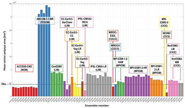
- Figure 2: are the models ordered in any particular way (e.g., based on resolution or the sea ice model used)?They are in alphabetical order.
- Line 218 ff. how could this value (the percentage of region where polynyas have opened for more than 25 years) be impacted by changing SIC/marginal ice zone conditions across models/years, e.g. in the mentioned East Siberian Sea?See similar comment made by Reviewer 2. We tested different thresholds as well as different time periods when conducting this study. In fact, at first we wrote the text with 35 winters, to get the most extreme behaviours. The text barely needed to be changed when we settled for the more average 25 winter value, only the percentages we quote. We are out of ideas regarding how to express uncertainty while also not having the table cover several pages, but would welcome suggestions.
- Line 235 ff. Trend: could it be related to retreating sea ice/“false“ detection of polynyas in the marginal ice zone? On page 9 you discuss the relation of SIA/SIE to polynya activity, I suggest you add a sentence about the relation of SIA/SIE trends and polynya trends if possible.This is an interesting comment. We did find in our previous study that the rate of false positives decreased along with SIA, when using the method on observations. We verified the relationship here on the models but found no across-model relationship between trend in SIA (or SIE) and the trend in polynya area nor with the mean polynya area. This further reinforces our hypothesis of a dynamical issue in the model, rather than a detection artefact.
We added a sentence summarising this point at the end of the paragraph that the reviewer refers to.
- Line 250 ff.: Clustering by sea ice model: I find this hard to tell from the Figure. I agree that a clustering of star symbols is visible for region 5 but I do not see it for region 6 as stated in line 252, for example. I suggest to either try to illustrate it more clearly in the figure (or an extra figure), maybe with semi-transparent symbols or a reduction to the two most common ice models, or by writing it in the text more explicitely (à la “clustering in the upper right quadrant…“). I find this especially important as part of the conclusions are drawn from this (see Abstract: „with most activity in the models whose thermodynamics scheme enhances ice growth/melt and least activity in models whose dynamics scheme dampens the influence of wind on ice“). Maybe you could indicate which sea ice model is used per ensemble in Figure 2.As recommended by the reviewer, we have added the sea ice model families (i.e. shorter names as on Fig 4, without the version number) to Figure 2.
We also added explicitly descriptions of where to find the models on Figure 4, as recommended by the reviewer:
“are often found together, most visibly by the Pacific inflow regions of the East Siberian (all of them are to the right), Chukchi (five out of seven in the top right corner) and Beaufort seas (all of them are to the bottom centre/left).”
- line 257: how short is short-lived?We rephrased as “Although polynyas usually last but a few days (Smith Jr and Barber, 2007)”. The exact duration depends on the region considered.
- Figure 5: please remove the plotting artefactIf it were easy to remove, we would have removed it before submission. Without entering into the gory details, we would either need to write a plotting script for every single model to make it look good, or spend many hours manually editing each image on paint.
- Figure 5, j): what is going on around 70°E? The white stripe looks suspicious.It is this model’s longitude grid origin; see previous comment.
- Section 3.2.: Using monthly SIC data comes with many drawbacks and the section nicely dissects them. However I find its size compared to the other sections disproportional for the (somewhat) expected results and recommendations (at least it distracted me a bit from the main story) and therefore I suggest to consider moving one of the two figures or even part of the text to the appendix.As recommended, we considered shortening this section but decided to leave it as it is. The first reason is that we were actually surprised by the results: not by the underestimation by the monthly models, but by the presence of a linear relationship between the two. The second reason is that few publications explicitly show how unrealistic the sea ice cover is in some of these models; it is easy to find a metric but rarely a map, so we prefer keeping it in the main text. Finally, since Reviewer 2 had several comments on this section, we did not want to look like we were trying to avoid addressing them by moving the text to the appendix.
- Section 4: Please define autumn and summer somewhere here or earlier (as e.g. summer sea ice thickness is often referred to in this section).The reviewer is correct: we defined the seasons in the table but not in the core of the text. Precision now added to the text.
- Line 319: „by definition where there is sea ice, polynyas can open“ This could be true also for other regions (?), consider adding a sentence why this is seen only for Svalbard.This is more of an intuition from looking at the sea ice in these models for too long. Having sea ice around Svalbard is the exception; having sea ice in the other regions is the norm. That is how this surprising correlation made sense to me. But maybe I am wrong and this correlation is a coincidence.
- Line 322 ff. and also line 394-396: Have you considered applying methods like time-lagged correlation analysis to back up your statement?I did and even started with time-lagged correlations, following the findings of Wong et al. (2026) that found different lags for air temperature vs wind, and even between the various wind component. The problem comes when applying this diagnostic to many different models, in several regions at the same time – there were results, but interpreting them was tricky. Since the objective of the manuscript is to find whether there are across-model similarities, we settled for this simplified approach. We nonetheless rephrased this part; see also the response to your comment line 404. We have also added text in the method section to clarify our approach and objectives.
- Line 348: Point 3, correlation to the equilibrium climate sensitivity: This hit me by surprise as the sentence starts with „To summarise“ but climate sensitivity has not been mentioned anywhere before. Please elaborate.We expanded this part, including our reasoning:
“A clue that the polynya bias is not linked to one specific, physical process, but rather caused by a deep model-dependent bias, e.g. in its treatment of thermodynamics, would be an across-model link between polynya bias and the model's equilibrium climate sensitivity (ECS). We do find a significant correlation of 0.76 between the ECS of Zelinka et al. (2020) and the pan-Arctic polynya area, with the caveat that there are only 9 models in common in our studies. That is, this link may not be robust, but it is encouraging.”
- Line 359 I suggest you add something like „ In sea ice models, it is the rheological formulation and roughness“ (or „ drag“)Reviewer 2 made extremely detailed comments on this point, including suggesting a reference that showed clearly the link between several model parameters and their impact on sea ice. We rephrased this part accordingly, including your suggestion as well.
- Line 391: As you consider December-March I would rephrase (it sounds as if warm air thins, that is, melts, the ice, I guess what is meant is that growth is slowed down). Another question I have here is whether the warmer winter air temperatures could be a consequence of larger polynya areas. Was this feedback considered?The sentence selected by the reviewer is actually a finding of Wong et al. (2026), not of this paper. However, since it is by the same team, I can answer: yes we did, see their Figure 7 and corresponding analysis in their section 4c. And it genuinely is warmer air leading the polynya opening, not the other way round. This is in fact one of the most exciting findings of Wong et al. (2026) in my opinion.
- Section 4.2. line. 404 ff. : I find the conclusions drawn here plausible, but I am missing a statement about the link of summer thickness and autumn thickness (how are they related/correlated?) or even something like a time-lagged correlation analysis to confirm that the thin summer ice is a consequence of large polynya activity while the thin autumn ice pre-conditiones for polynya opening.This is a fair point, especially since we have the means to verify this claim. Long story short, the autocorrelation of the sea ice is too strong to clearly distinguish whether previous or following year’s ice is the cause vs the consequence. That is, we find many strong correlations for all combinations of seasons, with no combination clearly dominating.
Reviewer 2 also asked us to verify the link between polynya activity and subsequent summer and likewise, although we do find many (negative) correlations between polynya are and sea ice thickness in the following summer, we do not find more and/or stronger correlations than with the previous summer. We rephrased this part accordingly.
- Section 5.1 line. 521. I would mention that this includes the “outlier“ model“Fair point. Comment added.
- Figure 7 and Figure 8: I suggest to use different shadings of blue and red to distinguish between the modelsWe modified the figures as recommended, using different shades of blue and red as well as different linestyles.
- Section 5.2. Line 464-465: “At the end of Section 4, we suspected that the models with the highest activity formed polynyas by melting the ice rather than by dynamic breaking due to strong winds.“ Where can I find this statement in Section 4? I understood there, that the thin autumn ice (which may or may not be a consequence of more melt, it could also be caused by less growth) preconditions the ice for dynamic breaking. Please explain. Is this based on the clustering by models? I think the study would benefit from a clearer distinction between air temperatures slowing growth and actual melt.As we now explicitly write in section 4, determining whether sea ice is actively melting or simply having a delayed growth is beyond the scope of this paper. This is another case where most likely, different models would have different behaviours in the different regions. It does matter for the preconditioning of the region for polynyas, which is why we instead took the approach of looking at the ocean profiles which are easier to interpret since they have less high variability (by definition – they are not available as daily output). And then, from the profiles, we can guess whether ice has melted or not. We rephrased to make the thought process clearer, and now explicitly name “sensible heat polynyas” as requested by Reviewer 2.
- Line 475: „most likely a result of how models open their polynya“. I am curious: could it be also a result of how models close their polynya? Is there a way for a model to dynamically close the polynya (without/little ice growth and thus, no dense-water generation)?In my opinion, based on our current effort to write a review on “real” Arctic polynyas, there is a lack of literature on how/why polynyas close. But if we take this as a thought exercise, one could in theory get larger-scale ice convergence that pushes the ice closed without having wind cooling at the polynya site itself – just a bit off. I would not be surprised if the Eurasian polynyas, in the models, behaved instead like the real-world Amerasian polynyas and require that a specific water mass be advected / upwelled, then modified by brine-enriched waters from the polynya, and only then sink as dense waters. But since these water masses are really poorly represented in CMIP6 (cf e.g. Heuzé et al. 2023), we would not get a clear answer.
- Line 495: „no consistent correlation at the individual model level“: this seems to contradict what you wrote in lines 366 ff or line 404 ff. Please explain.The reviewer is right, this sentence is confusing and contradicts section 4.2. We removed it.
- Line 502: „Our results do suggest however that polynya misrepresentation in CMIP6, in particular their too low frequency, may be caused by a reduced effect of wind on ice in climate models“. Please elaborate on this a bit more as this was not my take-away message from section 4. 2. For example, what makes you believe the effect is reduced?We made this point more explicit:
“Our results however show a lack of across-model relationship between wind and polynya activity, i.e. thermodynamics does not only matter for preconditioning but is also the trigger.”
And later:
“That is, CMIP6 models seem to be opening sensible heat polynyas in the Arctic, where all observed polynyas are latent-heat or hybrid”
- Line 514: „further suggesting (…) sea ice melt …“: Here, my comment refers more to the previous comment on lines 464 ff.: where was it stated that sea ice indeed melts in the models for polynyas to form? From my understanding of the section 4, the ice thickness is important but this is not necessarily a consequence of more melt. However I agree that the fresh water in the ocean models suggest it.See detailed response to the earlier comment referring to section 5.2.
- Figure A3 caption: I am not sure I understood the red arrows („point in the direction of its polynya area“), does it mean the values are outside of the x-axis limits?Yes; this model is an outlier, its value lies outside of the x-axis range.
technical:
- Consistent writing of Section vs. sectionVerified and corrected.
- Table 1: more complete if sivol is added in „comment“ columnWe use the comment section for exceptions to the “standard” set of variables, which we consider sivol to be one of.
- line 146 missing „and“Added.
- line 154: refer to figure numberIf we did so we would have to refer to Figure 3 before having referred to Figure 2. This is why we are using section numbers instead.
- line 426 typo „because of“Corrected.
Citation: https://doi.org/10.5194/egusphere-2026-901-AC1
-
AC1: 'Reply on RC1', Céline Heuzé, 11 May 2026
-
RC2: 'Comment on egusphere-2026-901', Anonymous Referee #2, 20 Apr 2026
This interesting and generally well-written manuscript is the first systematic study of CMIP model performance in terms of the Arctic polynyas, including their area and evolution. The topic and scope are suitable for the Cryosphere journal. However, there are some issues that the authors should address before I can recommend the publication of the manuscript in the journal. I list these points next in no particular order.
- line 61. I suppose 'the threshold' is based on sea-ice concentration. That should be clarified.
- lines 73-74. '(Brodzik et al. 2012)'
- line 110. Are the 'large errors' compared to observed sea-ice thickness?
- line 121. Here, the definition of sivol should be clarified. I suppose it is the sea-ice volume [m**3/m**2] in a grid cell per unit area, so that the mean sea-ice thickness in a grid cell is sivol divided by sea-ice concentration.
- line 122. Explain what 'unreliable' daily sea-ice thickness means.
- line 125. Is the ice density in these models constant?
- Table 1. Column 2 indicates the model horizontal resolution in square kilometres. But the models' grid cell area is not constant. Is the value presented the largest grid cell area north of 70 N?
- Table 1. Column 3 lists the sea-ice model components, but is quite confusing in places. For example, what is the difference between '~CICE', 'CICE' and 'CICE5'? Optimally, precise versions of LIM, CICE and COCO should be listed.
- line 172. I wonder how much difference the results would be when using single-model ensemble means instead of the first member. What would be the ensemble spread?
- line 190. This subsection title is confusing.
- line 195. Even though CanESM5 and NESM3 use the same ocean model NEMO, with nearly the same version (3.4.1 and 3.4), their sea-ice models differ. This difference could cause the bias.
- line 207. 'seasonally ice covered area' is a confusing term in this context. Do you mean Marginal Ice Zone (MIZ)?
- line 208. The claim that 'in observations there are polynyas in the permanent ice pack' seems misleading as the coastal regions, e.g. in the continental shelf, where winter polynyas occur, become ice-free in summer, so their ice-cover is not permanent. Would inner pack ice be a better expression?
- lines 213-215. Despite using the MIZ classification method, the data still contain noise from the MIZ, which the authors claim is unavoidable. This raises the question of why then use the MIZ classification methods at all?
- Figure 3. Just north of Region 1 and Svalbard lies an active polynya region that was excluded. Wouldn't it make sense to include it in the analysis by extending Region 1 northward?
- Section 3.2, general comment. Based on some earlier studies, in winter, the MIZ area is underestimated and the pack area is overestimated (e.g., Chevallier et al. 2017). Could such a shortcoming affect the CMIP model polynya evolution and extent?
- line 232. Which eight models underestimate the frequent-opening areas? This might be useful information.
- line 234. Which locations (referring to 'too many locations')?
- line 241. Is 'the 45-year mean bias' in the polynya area?
- line 252. Seems that the LIM models are in fact quite scattered in Fig. 4 in the Chukchi Sea.
- Table 2. How robust is the test limit: more than 25 out of 45 winters? What if you change that to 20 or 30? Percentages in the table and text are expressed with a rather high accuracy. How meaningful are the differences between the models? When are they statistically significant?
- In Figure 5 some panel labels are greek letters which is strange.
- In Figure 6, are all correlations significant at the 95% level, as there are no NaNs? What about regression slopes, what are they confidence limits? Seems that in panel 4. Lap, the regression may not be significant.
- line 321. 'and often with a stronger value'
- line 325-328. To confirm this, you should calculate correlations between the polynya area and the sea-ice thickness in the following summer.
- lines 329-331. These claims seem subjective. For example, the FJL correlation is -0.66 in JJA and -0.69 in DJF. Is this difference truly significant or a result of chance?
- line 340. Mention the sea-ice concentration threshold value. Is it 0.8?
- Table 3. Calling sivol 'the mean sea-ice thickness' is obscure. Use the term 'effective sea-ice thickness' or 'the sea-ice volume per unit area' or similar.
- line 359. In sea-ice models, not only the rheology matters, but also the form and skin drag at the air-ice and ice-ocean interfaces, plus atmospheric and oceanic boundary layer stratifications and mixing parametrisations. The importance of rheology is comparatively small when the sea-ice concentration is low, say below 0.7.
- line 360. The EVP rheology implemented in CICE, and actually also in LIM2/3, produces practically similar results to the VP rheology. The elastic waves were added for a faster numerical solution (Hunke & Dukowicz 1997). But there are other more important differences between CICE and LIM. In fact, in LIM2, there is no sub-grid-scale sea-ice thickness distribution, unlike in CICE and LIM3.
- Section 4.2. The analysis related to winds is really confusing. First, it is quite unfriendly for a reader to go and look for values from tables in the Appendices. Could the key findings be visualised e.g. in a bar plot or similar? It is also not convincing to separate the analysis between winds and temperatures. Instead, cold and warm air advection cases should be compared. For example, cyclones from the Atlantic bring in warm air and strong winds, which have entirely different effects on polynyas than cold air off-ice or off-land advection.
- line 399. Also, FJL, Kara and Chuk correlation with T2m in SON in Table 3. Why not mention them?
- line 400. 'the absolute value of the correlation'
- line 404. I do not think it is justified to call these relationships strong.
- line 407. An explanation for why warmer models have thinner ice in autumn is that when the air temperature is warmer, but below zero, the ice growth is slower.
- line 409. 'polynya area is evident, but lack'
- line 434. Makes sense that there is no sea-ice production in these modelled polynyas.
- line 465. 'fresh and warm waters.' This finding could be backed up by theory and you could mention that instead of latent heat polynyas, the models simulate sensible heat polynyas.
- lines 496-499. As mentioned before, see the one related to line 359, this explanation appears implausible.
Literature:
- Chevallier, M. et al.: Intercomparison of the Arctic sea ice cover in global ocean–sea ice reanalyses from the ORA-IP project, Climate Dynamics, 49, 1107–1136, https://doi.org/10.1007/s00382-016-2985-y, 2017.
- Hunke, E. C. and Dukowicz, J. K.: An Elastic–Viscous–Plastic Model for Sea Ice Dynamics, Journal of Physical Oceanography, 27, 1849–1867, https://doi.org/10.1175/1520-0485(1997)027%253C1849:AEVPMF%253E2.0.CO;2, 1997.
Citation: https://doi.org/10.5194/egusphere-2026-901-RC2 -
AC2: 'Reply on RC2', Céline Heuzé, 11 May 2026
We thank the reviewer for the time they spent reading and commenting on our paper. We have addressed all their comments, as detailed below. The contribution of the reviewer has been acknowledged in the acknowledgement section:
“We thank the two anonymous reviewers whose suggestions improved the manuscript”.
There are some issues that the authors should address before I can recommend the publication of the manuscript in the journal. I list these points next in no particular order.
- line 61. I suppose 'the threshold' is based on sea-ice concentration. That should be clarified.
Added “sea ice concentration or thickness”
- lines 73-74. '(Brodzik et al. 2012)'
Corrected
- line 110. Are the 'large errors' compared to observed sea-ice thickness?
Yes, as well as unrealistic values (e.g. thickness of more than 30 m). We added “compared to observations”.
- line 121. Here, the definition of sivol should be clarified. I suppose it is the sea-ice volume [m**3/m**2] in a grid cell per unit area, so that the mean sea-ice thickness in a grid cell is sivol divided by sea-ice concentration.
No, as we already explain, sivol is in fact the thickness computed as the volume divided by the area. Note that the variable long name is “sea ice thickness”. We suspect that this confusing choice of short name is to distinguish it from the thickness computed as the floe thickness, “sithick”. We rephrased our description of sivol.
- line 122. Explain what 'unreliable' daily sea-ice thickness means.
It was a polite version of the “large errors” of two comments ago. We rephrased as “has large errors, as we described above”
- line 125. Is the ice density in these models constant?
As far as we understand, yes.
- Table 1. Column 2 indicates the model horizontal resolution in square kilometres. But the models' grid cell area is not constant. Is the value presented the largest grid cell area north of 70 N?
No, it is the area north of 70N, in km^2, divided by the number of grid cells that the model has north of 70N. We now explain this in the table caption.
- Table 1. Column 3 lists the sea-ice model components, but is quite confusing in places. For example, what is the difference between '~CICE', 'CICE' and 'CICE5'? Optimally, precise versions of LIM, CICE and COCO should be listed.
Yes, this would be optimum. It would be great if model description papers systematically, explicitly listed their model version for all their components, or if at least if these were indicated on the ESGF description page meant for that exact purpose. Unfortunately, this is often not described, so this column represents the extent of the information available.
We expanded the table caption as “Sea ice component and version, when indicated in the reference (~ means similar to, according to the reference)”.- line 172. I wonder how much difference the results would be when using single-model ensemble means instead of the first member. What would be the ensemble spread?
For our values, this is addressed in section 3.1, including Figure 2 and appendix Figure A1, where we show that the ensemble spread was negligible compared to the inter-model spread. For comparison with the values of Tian et al. (2024), unless we force them to redo their study with an ensemble instead of the first member, we prefer using the first ensemble member too.
- line 190. This subsection title is confusing.
We renamed our section. If the reviewer still finds it confusing, we would appreciate suggestions for alternative titles.
- line 195. Even though CanESM5 and NESM3 use the same ocean model NEMO, with nearly the same version (3.4.1 and 3.4), their sea-ice models differ. This difference could cause the bias.
Yes, this is what we argue in section 4.1. We have added a teaser following the reviewer’s comment.
- line 207. 'seasonally ice covered area' is a confusing term in this context. Do you mean Marginal Ice Zone (MIZ)?
No, we mean the area between the summer extent and the winter extent, i.e. only ice-covered in winter. We rephrased.
- line 208. The claim that 'in observations there are polynyas in the permanent ice pack' seems misleading as the coastal regions, e.g. in the continental shelf, where winter polynyas occur, become ice-free in summer, so their ice-cover is not permanent. Would inner pack ice be a better expression?
No, not all coastal regions become ice-free in summer. Or at least they used not to; nothing is really permanent anymore these days, even the “last ice area” is starting to have polynyas. We rephrased using the term you suggested.
- lines 213-215. Despite using the MIZ classification method, the data still contain noise from the MIZ, which the authors claim is unavoidable. This raises the question of why then use the MIZ classification methods at all?
It is way worse without the MIZ filter. That is why that filter was developed in the first place: we got the Unet algorithm to the point where it returned no false negative, but with the drawback that it returned many false positives. This is detailed and illustrated in Heuzé and Wong (2025).
- Figure 3. Just north of Region 1 and Svalbard lies an active polynya region that was excluded. Wouldn't it make sense to include it in the analysis by extending Region 1 northward?
Our region definition is consistent with Preusser et al. (2016), Ohshima et al. (2016), and Wong et al. (2026), i.e. the three most recent studies of pan-Arctic and regional polynya activity in the Arctic. If we changed the region definition, we would not be able to directly compare to their findings.
- Section 3.2, general comment. Based on some earlier studies, in winter, the MIZ area is underestimated and the pack area is overestimated (e.g., Chevallier et al. 2017). Could such a shortcoming affect the CMIP model polynya evolution and extent?
We thank the reviewer for bringing this publication to our attention. We did not find the results that the reviewer highlights – the authors rather insist on the dipole Beaufort Gyre / North Pole, but we now have even more parameers to discuss in section 4: numbers of sea ice thickness classes, air-ice drag coefficient, ice-ocean drag coefficient, and ice strength.
- line 232. Which seven models underestimate the frequent-opening areas? This might be useful information.
We added the name of these seven models, as well as those of the 13 in the second half of that sentence.
- line 234. Which locations (referring to 'too many locations')?
This refers to the percentage / metric we spent that and the previous paragraph describing. We are not talking about any specific location but about that metric.
- line 241. Is 'the 45-year mean bias' in the polynya area?
Yes, as the sentence already read in the previous version, but we have now made it even more explicit.
- line 252. Seems that the LIM models are in fact quite scattered in Fig. 4 in the Chukchi Sea.
Five out of seven are quite close to each other, and our phrasing was already very soft: “appears”, “often”, “might”. We nonetheless rephrased, following a comment by Reviewer 1.
- Table 2. How robust is the test limit: more than 25 out of 45 winters? What if you change that to 20 or 30? Percentages in the table and text are expressed with a rather high accuracy. How meaningful are the differences between the models? When are they statistically significant?
See similar comment made by Reviewer 1. We tested different thresholds as well as different time periods when conducting this study. In fact, at first we wrote the text with 35 winters, to get the most extreme behaviours. The text barely needed to be changed when we settled for the more average 25 winter value, only the percentages we quote. We are out of ideas regarding how to express uncertainty while also not having the table cover several pages, but would welcome suggestions.
- In Figure 5 some panel labels are greek letters which is strange.
That is because there are 35 monthly models but only 26 letters in the standard English alphabet. We completed with the Greek alphabet.
- In Figure 6, are all correlations significant at the 95% level, as there are no NaNs? What about regression slopes, what are they confidence limits? Seems that in panel 4. Lap, the regression may not be significant.
Yes they are all significant at 95%; that is why there are no NaNs.
Regarding the regression slopes, the significance of the regression and the correlation coefficient are evaluated simultaneously in this analysis, and thus they share the same significance level. Therefore, all displayed regression slopes are also significant at the 95% level, including the regression shown in panel 4. Lap.- line 321. 'and often with a stronger value'
Rephrased as suggested.
- line 325-328. To confirm this, you should calculate correlations between the polynya area and the sea-ice thickness in the following summer.
That’s a fair point. And although we do find many (negative) correlations between polynya area and sea ice thickness in the following summer, we do not find more and/or stronger correlations than with the previous summer. We did not add the values to Appendix Table A5 which is already full page. We instead rephrased this part, also following a comment on sea ice autocorrelation by Reviewer 1.
- lines 329-331. These claims seem subjective. For example, the FJL correlation is -0.66 in JJA and -0.69 in DJF. Is this difference truly significant or a result of chance?
We rephrased to make the claim less strong: “in the Chukchi sea, it is strongest with the winter thickness; in Franz Josef Land, it is nearly equally strong with both seasons”
- line 340. Mention the sea-ice concentration threshold value. Is it 0.8?
Now mentioned. Athanase et al. (2025) say “approximately 80%”, yes.
- Table 3. Calling sivol 'the mean sea-ice thickness' is obscure. Use the term 'effective sea-ice thickness' or 'the sea-ice volume per unit area' or similar.
No, sivol is called “the sea ice thickness” (not our choice, this is its ESGF long name), and we take its mean. We rephrased the table caption to clarify this.
- line 359. In sea-ice models, not only the rheology matters, but also the form and skin drag at the air-ice and ice-ocean interfaces, plus atmospheric and oceanic boundary layer stratifications and mixing parametrisations. The importance of rheology is comparatively small when the sea-ice concentration is low, say below 0.7.
And line 360. The EVP rheology implemented in CICE, and actually also in LIM2/3, produces practically similar results to the VP rheology. The elastic waves were added for a faster numerical solution (Hunke & Dukowicz 1997). But there are other more important differences between CICE and LIM. In fact, in LIM2, there is no sub-grid-scale sea-ice thickness distribution, unlike in CICE and LIM3.
We rephrased this part. We addressed these two comments by referring to the Chevallier et al. (2017) publication that the reviewer recommended earlier, and correcting our comment about EVP following the reviewer’s clarification. See also our earlier response to the reviewer’s comment asking for the model version number to be provided. Note also that since we are interested in the opening of polynyas, we investigate why the model moves away from a consolidated pack ice with concentrations usually higher than 0.7, so rheology does matter.
- Section 4.2. The analysis related to winds is really confusing. First, it is quite unfriendly for a reader to go and look for values from tables in the Appendices. Could the key findings be visualised e.g. in a bar plot or similar? It is also not convincing to separate the analysis between winds and temperatures. Instead, cold and warm air advection cases should be compared. For example, cyclones from the Atlantic bring in warm air and strong winds, which have entirely different effects on polynyas than cold air off-ice or off-land advection.
The objective of this manuscript is not to conduct a process study, which we would not be able to do anyway since we do not have output at the right temporal resolution, but to try and find a link between polynya biases and other model biases, to inform modellers that would be interested in improving their sea ice representation. We find no such link with the winds, so rather than directly concluding that the dynamics are completely wrong in the models, we give them another chance by investigating biases at the timeseries, individual model level. There are no single key findings to highlight; the key finding is that “it depends”, hence the many long tables that, out of sympathy for most readers, we kicked to the appendix.
We have added text in the method section to clarify the objective of the study and our choice of methods.
As for warm air intrusions, although we agree that this would be very interesting as a stand-alone study, ideally in observations first, such high-frequency compound events are beyond the scope of this study.
- line 399. Also, FJL, Kara and Chuk correlation with T2m in SON in Table 3. Why not mention them?
The sentence is about regions where there only is correlation with the autumn, not with the other seasons. In FJL, Kara and Chuk, there are correlations in at least another season; they are not the topic of this sentence.
- line 400. 'the absolute value of the correlation'
Rephrased as suggested.
- line 404. I do not think it is justified to call these relationships strong.
Changed “strong” into “significant”.
- line 407. An explanation for why warmer models have thinner ice in autumn is that when the air temperature is warmer, but below zero, the ice growth is slower.
This is what we had tried to convey. We rephrased, also based on a similar comment by Reviewer 1.
- line 409. 'polynya area is evident, but lack'
This sentence has been removed in response to the previous and earlier comments.
- line 434. Makes sense that there is no sea-ice production in these modelled polynyas.
We are not sure which sentence the reviewer is commenting on, but we are glad they agree with our overall findings.
- line 465. 'fresh and warm waters.' This finding could be backed up by theory and you could mention that instead of latent heat polynyas, the models simulate sensible heat polynyas.
This joins a similar comment by Reviewer 1. We rephrased this part to address their comment, but added a reference to sensible heat polynyas as suggested.
- lines 496-499. As mentioned before, see the one related to line 359, this explanation appears implausible.
Rephrased using also the findings of Chevallier et al. (2017), as recommended by the reviewer.
Citation: https://doi.org/10.5194/egusphere-2026-901-AC2


Interactive discussion
Status: closed
-
RC1: 'Comment on egusphere-2026-901', Anonymous Referee #1, 14 Apr 2026
I have reviewed the manuscript titled „Winter Arctic polynyas in CMIP6 models“ by Heuzé et al..
Their study evaluates and compares how current (CMIP6) climate models represent polynyas. To my knowledge, such a study was missing for the Arctic (but exists for the Antarctic), despite the important role polynyas play in the Arctic climate system (e.g., sea ice production, biological hotspots/biodiversity, coupling of ocean to the atmosphere, etc.).The authors use a newly developed polynya detection method (Wong et al., 2026) based on sea ice concentration (SIC) to compare yearly/winter mean polynya area, frequency and trends across models and against satellite observations. The writing is clear and the methodology is sound as the authors also discuss (the limits of) their detection method (e.g. testing different thresholds, the limitations in the marginal ice zone, the dependence of the results on grid resolution, etc.) as well as their statistical diagnostics (e.g. using cumulative polynya area instead of winter mean area, using monthly instead of daily SIC data, etc.). Data and methods are well described (Section 2) and data and source code are mostly openly available (or will be made available soon). Also, the results sections benefit from a clear structure with summaries at the end of subsections. The potential causes of biases are thoroughly and concisely analyzed, using correlations as main (and available) tool, and discussed in Section 4. The impact on the ocean (deep) water representation, a question motivating this study, is exemplarily discussed with well chosen indicators of the water column.
The figures and tables are overall well done.
The last chapter summarizes the main findings and new insights of the study and provides an outlook on how to improve the representation of polynyas in climate model but could benefit from minor improvements. Overall, the study is of high quality and a step towards understanding how polynya (processes) are biased in climate models.Below, I provide more specific comments and suggestions for improvement. I am highlighting the comments I find most important as bold:
- Figure 2: are the models ordered in any particular way (e.g., based on resolution or the sea ice model used)?
- Line 218 ff. how could this value (the percentage of region where polynyas have opened for more than 25 years) be impacted by changing SIC/marginal ice zone conditions across models/years, e.g. in the mentioned East Siberian Sea?
- Line 235 ff. Trend: could it be related to retreating sea ice/“false“ detection of polynyas in the marginal ice zone? On page 9 you discuss the relation of SIA/SIE to polynya activity, I suggest you add a sentence about the relation of SIA/SIE trends and polynya trends if possible.
- Line 250 ff.: Clustering by sea ice model: I find this hard to tell from the Figure. I agree that a clustering of star symbols is visible for region 5 but I do not see it for region 6 as stated in line 252, for example. I suggest to either try to illustrate it more clearly in the figure (or an extra figure), maybe with semi-transparent symbols or a reduction to the two most common ice models, or by writing it in the text more explicitely (à la “clustering in the upper right quadrant…“). I find this especially important as part of the conclusions are drawn from this (see Abstract: „with most activity in the models whose thermodynamics scheme enhances ice growth/melt and least activity in models whose dynamics scheme dampens the influence of wind on ice“). Maybe you could indicate which sea ice model is used per ensemble in Figure 2.
- line 257: how short is short-lived?
- Figure 5: please remove the plotting artefact
- Figure 5, j): what is going on around 70°E? The white stripe looks suspicious.
- Section 3.2.: Using monthly SIC data comes with many drawbacks and the section nicely dissects them. However I find its size compared to the other sections disproportional for the (somewhat) expected results and recommendations (at least it distracted me a bit from the main story) and therefore I suggest to consider moving one of the two figures or even part of the text to the appendix.
- Section 4: Please define autumn and summer somewhere here or earlier (as e.g. summer sea ice thickness is often referred to in this section).
- Line 319: „by definition where there is sea ice, polynyas can open“ This could be true also for other regions (?), consider adding a sentence why this is seen only for Svalbard.
- Line 322 ff. and also line 394-396: Have you considered applying methods like time-lagged correlation analysis to back up your statement?
- Line 348: Point 3, correlation to the equilibrium climate sensitivity: This hit me by surprise as the sentence starts with „To summarise“ but climate sensitivity has not been mentioned anywhere before. Please elaborate.
- Line 359 I suggest you add something like „ In sea ice models, it is the rheological formulation and roughness“ (or „ drag“)
- Line 391: As you consider December-March I would rephrase (it sounds as if warm air thins, that is, melts, the ice, I guess what is meant is that growth is slowed down). Another question I have here is whether the warmer winter air temperatures could be a consequence of larger polynya areas. Was this feedback considered?
- Section 4.2. line. 404 ff. : I find the conclusions drawn here plausible, but I am missing a statement about the link of summer thickness and autumn thickness (how are they related/correlated?) or even something like a time-lagged correlation analysis to confirm that the thin summer ice is a consequence of large polynya activity while the thin autumn ice pre-conditiones for polynya opening.
- Section 5.1 line. 521. I would mention that this includes the “outlier“ model“
- Figure 7 and Figure 8: I suggest to use different shadings of blue and red to distinguish between the models
- Section 5.2. Line 464-465: “At the end of Section 4, we suspected that the models with the highest activity formed polynyas by melting the ice rather than by dynamic breaking due to strong winds.“ Where can I find this statement in Section 4? I understood there, that the thin autumn ice (which may or may not be a consequence of more melt, it could also be caused by less growth) preconditions the ice for dynamic breaking. Please explain. Is this based on the clustering by models? I think the study would benefit from a clearer distinction between air temperatures slowing growth and actual melt.
- Line 475: „mosty likely a result of how models open their polynya“. I am curious: could it be also a result of how models close their polynya? Is there a way for a model to dynamically close the polynya (without/little ice growth and thus, no dense-water generation)?
- Line 495: „no consistent correlation at the individual model level“: this seems to contradict what you wrote in lines 366 ff or line 404 ff. Please explain.
- Line 502: „Our results do suggest however that polynya misrepresentation in CMIP6, in particular their too low frequency, may be caused by a reduced effect of wind on ice in climate models“. Please elaborate on this a bit more as this was not my take-away message from section 4. 2. For example, what makes you believe the effect is reduced?
- Line 514: „further suggesting (…) sea ice melt …“: Here, my comment refers more to the previous comment on lines 464 ff.: where was it stated that sea ice indeed melts in the models for polynyas to form? From my understanding of the section 4, the ice thickness is important but this is not necessarily a consequence of more melt. However I agree that the fresh water in the ocean models suggest it.
- Figure A3 caption: I am not sure I understood the red arrows („point in the direction of its polynya area“), does it mean the values are outside of the x-axis limits?technical:
- Consistent writing of Section vs. section
- Table 1: more complete if sivol is added in „comment“ column
- line 146 missing „and“
- line 154: refer to figure number
- line 426 typo „because of“Citation: https://doi.org/10.5194/egusphere-2026-901-RC1 -
AC1: 'Reply on RC1', Céline Heuzé, 11 May 2026
We thank the reviewer for the time they spent reading and commenting on our paper. We have addressed all their comments, as detailed below. The contribution of the reviewer has been acknowledged in the acknowledgement section:
“We thank the two anonymous reviewers whose suggestions improved the manuscript”.
Below, I provide more specific comments and suggestions for improvement. I am highlighting the comments I find most important as bold:
- Figure 2: are the models ordered in any particular way (e.g., based on resolution or the sea ice model used)?They are in alphabetical order.
- Line 218 ff. how could this value (the percentage of region where polynyas have opened for more than 25 years) be impacted by changing SIC/marginal ice zone conditions across models/years, e.g. in the mentioned East Siberian Sea?See similar comment made by Reviewer 2. We tested different thresholds as well as different time periods when conducting this study. In fact, at first we wrote the text with 35 winters, to get the most extreme behaviours. The text barely needed to be changed when we settled for the more average 25 winter value, only the percentages we quote. We are out of ideas regarding how to express uncertainty while also not having the table cover several pages, but would welcome suggestions.
- Line 235 ff. Trend: could it be related to retreating sea ice/“false“ detection of polynyas in the marginal ice zone? On page 9 you discuss the relation of SIA/SIE to polynya activity, I suggest you add a sentence about the relation of SIA/SIE trends and polynya trends if possible.This is an interesting comment. We did find in our previous study that the rate of false positives decreased along with SIA, when using the method on observations. We verified the relationship here on the models but found no across-model relationship between trend in SIA (or SIE) and the trend in polynya area nor with the mean polynya area. This further reinforces our hypothesis of a dynamical issue in the model, rather than a detection artefact.
We added a sentence summarising this point at the end of the paragraph that the reviewer refers to.
- Line 250 ff.: Clustering by sea ice model: I find this hard to tell from the Figure. I agree that a clustering of star symbols is visible for region 5 but I do not see it for region 6 as stated in line 252, for example. I suggest to either try to illustrate it more clearly in the figure (or an extra figure), maybe with semi-transparent symbols or a reduction to the two most common ice models, or by writing it in the text more explicitely (à la “clustering in the upper right quadrant…“). I find this especially important as part of the conclusions are drawn from this (see Abstract: „with most activity in the models whose thermodynamics scheme enhances ice growth/melt and least activity in models whose dynamics scheme dampens the influence of wind on ice“). Maybe you could indicate which sea ice model is used per ensemble in Figure 2.As recommended by the reviewer, we have added the sea ice model families (i.e. shorter names as on Fig 4, without the version number) to Figure 2.
We also added explicitly descriptions of where to find the models on Figure 4, as recommended by the reviewer:
“are often found together, most visibly by the Pacific inflow regions of the East Siberian (all of them are to the right), Chukchi (five out of seven in the top right corner) and Beaufort seas (all of them are to the bottom centre/left).”
- line 257: how short is short-lived?We rephrased as “Although polynyas usually last but a few days (Smith Jr and Barber, 2007)”. The exact duration depends on the region considered.
- Figure 5: please remove the plotting artefactIf it were easy to remove, we would have removed it before submission. Without entering into the gory details, we would either need to write a plotting script for every single model to make it look good, or spend many hours manually editing each image on paint.
- Figure 5, j): what is going on around 70°E? The white stripe looks suspicious.It is this model’s longitude grid origin; see previous comment.
- Section 3.2.: Using monthly SIC data comes with many drawbacks and the section nicely dissects them. However I find its size compared to the other sections disproportional for the (somewhat) expected results and recommendations (at least it distracted me a bit from the main story) and therefore I suggest to consider moving one of the two figures or even part of the text to the appendix.As recommended, we considered shortening this section but decided to leave it as it is. The first reason is that we were actually surprised by the results: not by the underestimation by the monthly models, but by the presence of a linear relationship between the two. The second reason is that few publications explicitly show how unrealistic the sea ice cover is in some of these models; it is easy to find a metric but rarely a map, so we prefer keeping it in the main text. Finally, since Reviewer 2 had several comments on this section, we did not want to look like we were trying to avoid addressing them by moving the text to the appendix.
- Section 4: Please define autumn and summer somewhere here or earlier (as e.g. summer sea ice thickness is often referred to in this section).The reviewer is correct: we defined the seasons in the table but not in the core of the text. Precision now added to the text.
- Line 319: „by definition where there is sea ice, polynyas can open“ This could be true also for other regions (?), consider adding a sentence why this is seen only for Svalbard.This is more of an intuition from looking at the sea ice in these models for too long. Having sea ice around Svalbard is the exception; having sea ice in the other regions is the norm. That is how this surprising correlation made sense to me. But maybe I am wrong and this correlation is a coincidence.
- Line 322 ff. and also line 394-396: Have you considered applying methods like time-lagged correlation analysis to back up your statement?I did and even started with time-lagged correlations, following the findings of Wong et al. (2026) that found different lags for air temperature vs wind, and even between the various wind component. The problem comes when applying this diagnostic to many different models, in several regions at the same time – there were results, but interpreting them was tricky. Since the objective of the manuscript is to find whether there are across-model similarities, we settled for this simplified approach. We nonetheless rephrased this part; see also the response to your comment line 404. We have also added text in the method section to clarify our approach and objectives.
- Line 348: Point 3, correlation to the equilibrium climate sensitivity: This hit me by surprise as the sentence starts with „To summarise“ but climate sensitivity has not been mentioned anywhere before. Please elaborate.We expanded this part, including our reasoning:
“A clue that the polynya bias is not linked to one specific, physical process, but rather caused by a deep model-dependent bias, e.g. in its treatment of thermodynamics, would be an across-model link between polynya bias and the model's equilibrium climate sensitivity (ECS). We do find a significant correlation of 0.76 between the ECS of Zelinka et al. (2020) and the pan-Arctic polynya area, with the caveat that there are only 9 models in common in our studies. That is, this link may not be robust, but it is encouraging.”
- Line 359 I suggest you add something like „ In sea ice models, it is the rheological formulation and roughness“ (or „ drag“)Reviewer 2 made extremely detailed comments on this point, including suggesting a reference that showed clearly the link between several model parameters and their impact on sea ice. We rephrased this part accordingly, including your suggestion as well.
- Line 391: As you consider December-March I would rephrase (it sounds as if warm air thins, that is, melts, the ice, I guess what is meant is that growth is slowed down). Another question I have here is whether the warmer winter air temperatures could be a consequence of larger polynya areas. Was this feedback considered?The sentence selected by the reviewer is actually a finding of Wong et al. (2026), not of this paper. However, since it is by the same team, I can answer: yes we did, see their Figure 7 and corresponding analysis in their section 4c. And it genuinely is warmer air leading the polynya opening, not the other way round. This is in fact one of the most exciting findings of Wong et al. (2026) in my opinion.
- Section 4.2. line. 404 ff. : I find the conclusions drawn here plausible, but I am missing a statement about the link of summer thickness and autumn thickness (how are they related/correlated?) or even something like a time-lagged correlation analysis to confirm that the thin summer ice is a consequence of large polynya activity while the thin autumn ice pre-conditiones for polynya opening.This is a fair point, especially since we have the means to verify this claim. Long story short, the autocorrelation of the sea ice is too strong to clearly distinguish whether previous or following year’s ice is the cause vs the consequence. That is, we find many strong correlations for all combinations of seasons, with no combination clearly dominating.
Reviewer 2 also asked us to verify the link between polynya activity and subsequent summer and likewise, although we do find many (negative) correlations between polynya are and sea ice thickness in the following summer, we do not find more and/or stronger correlations than with the previous summer. We rephrased this part accordingly.
- Section 5.1 line. 521. I would mention that this includes the “outlier“ model“Fair point. Comment added.
- Figure 7 and Figure 8: I suggest to use different shadings of blue and red to distinguish between the modelsWe modified the figures as recommended, using different shades of blue and red as well as different linestyles.
- Section 5.2. Line 464-465: “At the end of Section 4, we suspected that the models with the highest activity formed polynyas by melting the ice rather than by dynamic breaking due to strong winds.“ Where can I find this statement in Section 4? I understood there, that the thin autumn ice (which may or may not be a consequence of more melt, it could also be caused by less growth) preconditions the ice for dynamic breaking. Please explain. Is this based on the clustering by models? I think the study would benefit from a clearer distinction between air temperatures slowing growth and actual melt.As we now explicitly write in section 4, determining whether sea ice is actively melting or simply having a delayed growth is beyond the scope of this paper. This is another case where most likely, different models would have different behaviours in the different regions. It does matter for the preconditioning of the region for polynyas, which is why we instead took the approach of looking at the ocean profiles which are easier to interpret since they have less high variability (by definition – they are not available as daily output). And then, from the profiles, we can guess whether ice has melted or not. We rephrased to make the thought process clearer, and now explicitly name “sensible heat polynyas” as requested by Reviewer 2.
- Line 475: „most likely a result of how models open their polynya“. I am curious: could it be also a result of how models close their polynya? Is there a way for a model to dynamically close the polynya (without/little ice growth and thus, no dense-water generation)?In my opinion, based on our current effort to write a review on “real” Arctic polynyas, there is a lack of literature on how/why polynyas close. But if we take this as a thought exercise, one could in theory get larger-scale ice convergence that pushes the ice closed without having wind cooling at the polynya site itself – just a bit off. I would not be surprised if the Eurasian polynyas, in the models, behaved instead like the real-world Amerasian polynyas and require that a specific water mass be advected / upwelled, then modified by brine-enriched waters from the polynya, and only then sink as dense waters. But since these water masses are really poorly represented in CMIP6 (cf e.g. Heuzé et al. 2023), we would not get a clear answer.
- Line 495: „no consistent correlation at the individual model level“: this seems to contradict what you wrote in lines 366 ff or line 404 ff. Please explain.The reviewer is right, this sentence is confusing and contradicts section 4.2. We removed it.
- Line 502: „Our results do suggest however that polynya misrepresentation in CMIP6, in particular their too low frequency, may be caused by a reduced effect of wind on ice in climate models“. Please elaborate on this a bit more as this was not my take-away message from section 4. 2. For example, what makes you believe the effect is reduced?We made this point more explicit:
“Our results however show a lack of across-model relationship between wind and polynya activity, i.e. thermodynamics does not only matter for preconditioning but is also the trigger.”
And later:
“That is, CMIP6 models seem to be opening sensible heat polynyas in the Arctic, where all observed polynyas are latent-heat or hybrid”
- Line 514: „further suggesting (…) sea ice melt …“: Here, my comment refers more to the previous comment on lines 464 ff.: where was it stated that sea ice indeed melts in the models for polynyas to form? From my understanding of the section 4, the ice thickness is important but this is not necessarily a consequence of more melt. However I agree that the fresh water in the ocean models suggest it.See detailed response to the earlier comment referring to section 5.2.
- Figure A3 caption: I am not sure I understood the red arrows („point in the direction of its polynya area“), does it mean the values are outside of the x-axis limits?Yes; this model is an outlier, its value lies outside of the x-axis range.
technical:
- Consistent writing of Section vs. sectionVerified and corrected.
- Table 1: more complete if sivol is added in „comment“ columnWe use the comment section for exceptions to the “standard” set of variables, which we consider sivol to be one of.
- line 146 missing „and“Added.
- line 154: refer to figure numberIf we did so we would have to refer to Figure 3 before having referred to Figure 2. This is why we are using section numbers instead.
- line 426 typo „because of“Corrected.
Citation: https://doi.org/10.5194/egusphere-2026-901-AC1
-
AC1: 'Reply on RC1', Céline Heuzé, 11 May 2026
-
RC2: 'Comment on egusphere-2026-901', Anonymous Referee #2, 20 Apr 2026
This interesting and generally well-written manuscript is the first systematic study of CMIP model performance in terms of the Arctic polynyas, including their area and evolution. The topic and scope are suitable for the Cryosphere journal. However, there are some issues that the authors should address before I can recommend the publication of the manuscript in the journal. I list these points next in no particular order.
- line 61. I suppose 'the threshold' is based on sea-ice concentration. That should be clarified.
- lines 73-74. '(Brodzik et al. 2012)'
- line 110. Are the 'large errors' compared to observed sea-ice thickness?
- line 121. Here, the definition of sivol should be clarified. I suppose it is the sea-ice volume [m**3/m**2] in a grid cell per unit area, so that the mean sea-ice thickness in a grid cell is sivol divided by sea-ice concentration.
- line 122. Explain what 'unreliable' daily sea-ice thickness means.
- line 125. Is the ice density in these models constant?
- Table 1. Column 2 indicates the model horizontal resolution in square kilometres. But the models' grid cell area is not constant. Is the value presented the largest grid cell area north of 70 N?
- Table 1. Column 3 lists the sea-ice model components, but is quite confusing in places. For example, what is the difference between '~CICE', 'CICE' and 'CICE5'? Optimally, precise versions of LIM, CICE and COCO should be listed.
- line 172. I wonder how much difference the results would be when using single-model ensemble means instead of the first member. What would be the ensemble spread?
- line 190. This subsection title is confusing.
- line 195. Even though CanESM5 and NESM3 use the same ocean model NEMO, with nearly the same version (3.4.1 and 3.4), their sea-ice models differ. This difference could cause the bias.
- line 207. 'seasonally ice covered area' is a confusing term in this context. Do you mean Marginal Ice Zone (MIZ)?
- line 208. The claim that 'in observations there are polynyas in the permanent ice pack' seems misleading as the coastal regions, e.g. in the continental shelf, where winter polynyas occur, become ice-free in summer, so their ice-cover is not permanent. Would inner pack ice be a better expression?
- lines 213-215. Despite using the MIZ classification method, the data still contain noise from the MIZ, which the authors claim is unavoidable. This raises the question of why then use the MIZ classification methods at all?
- Figure 3. Just north of Region 1 and Svalbard lies an active polynya region that was excluded. Wouldn't it make sense to include it in the analysis by extending Region 1 northward?
- Section 3.2, general comment. Based on some earlier studies, in winter, the MIZ area is underestimated and the pack area is overestimated (e.g., Chevallier et al. 2017). Could such a shortcoming affect the CMIP model polynya evolution and extent?
- line 232. Which eight models underestimate the frequent-opening areas? This might be useful information.
- line 234. Which locations (referring to 'too many locations')?
- line 241. Is 'the 45-year mean bias' in the polynya area?
- line 252. Seems that the LIM models are in fact quite scattered in Fig. 4 in the Chukchi Sea.
- Table 2. How robust is the test limit: more than 25 out of 45 winters? What if you change that to 20 or 30? Percentages in the table and text are expressed with a rather high accuracy. How meaningful are the differences between the models? When are they statistically significant?
- In Figure 5 some panel labels are greek letters which is strange.
- In Figure 6, are all correlations significant at the 95% level, as there are no NaNs? What about regression slopes, what are they confidence limits? Seems that in panel 4. Lap, the regression may not be significant.
- line 321. 'and often with a stronger value'
- line 325-328. To confirm this, you should calculate correlations between the polynya area and the sea-ice thickness in the following summer.
- lines 329-331. These claims seem subjective. For example, the FJL correlation is -0.66 in JJA and -0.69 in DJF. Is this difference truly significant or a result of chance?
- line 340. Mention the sea-ice concentration threshold value. Is it 0.8?
- Table 3. Calling sivol 'the mean sea-ice thickness' is obscure. Use the term 'effective sea-ice thickness' or 'the sea-ice volume per unit area' or similar.
- line 359. In sea-ice models, not only the rheology matters, but also the form and skin drag at the air-ice and ice-ocean interfaces, plus atmospheric and oceanic boundary layer stratifications and mixing parametrisations. The importance of rheology is comparatively small when the sea-ice concentration is low, say below 0.7.
- line 360. The EVP rheology implemented in CICE, and actually also in LIM2/3, produces practically similar results to the VP rheology. The elastic waves were added for a faster numerical solution (Hunke & Dukowicz 1997). But there are other more important differences between CICE and LIM. In fact, in LIM2, there is no sub-grid-scale sea-ice thickness distribution, unlike in CICE and LIM3.
- Section 4.2. The analysis related to winds is really confusing. First, it is quite unfriendly for a reader to go and look for values from tables in the Appendices. Could the key findings be visualised e.g. in a bar plot or similar? It is also not convincing to separate the analysis between winds and temperatures. Instead, cold and warm air advection cases should be compared. For example, cyclones from the Atlantic bring in warm air and strong winds, which have entirely different effects on polynyas than cold air off-ice or off-land advection.
- line 399. Also, FJL, Kara and Chuk correlation with T2m in SON in Table 3. Why not mention them?
- line 400. 'the absolute value of the correlation'
- line 404. I do not think it is justified to call these relationships strong.
- line 407. An explanation for why warmer models have thinner ice in autumn is that when the air temperature is warmer, but below zero, the ice growth is slower.
- line 409. 'polynya area is evident, but lack'
- line 434. Makes sense that there is no sea-ice production in these modelled polynyas.
- line 465. 'fresh and warm waters.' This finding could be backed up by theory and you could mention that instead of latent heat polynyas, the models simulate sensible heat polynyas.
- lines 496-499. As mentioned before, see the one related to line 359, this explanation appears implausible.
Literature:
- Chevallier, M. et al.: Intercomparison of the Arctic sea ice cover in global ocean–sea ice reanalyses from the ORA-IP project, Climate Dynamics, 49, 1107–1136, https://doi.org/10.1007/s00382-016-2985-y, 2017.
- Hunke, E. C. and Dukowicz, J. K.: An Elastic–Viscous–Plastic Model for Sea Ice Dynamics, Journal of Physical Oceanography, 27, 1849–1867, https://doi.org/10.1175/1520-0485(1997)027%253C1849:AEVPMF%253E2.0.CO;2, 1997.
Citation: https://doi.org/10.5194/egusphere-2026-901-RC2 -
AC2: 'Reply on RC2', Céline Heuzé, 11 May 2026
We thank the reviewer for the time they spent reading and commenting on our paper. We have addressed all their comments, as detailed below. The contribution of the reviewer has been acknowledged in the acknowledgement section:
“We thank the two anonymous reviewers whose suggestions improved the manuscript”.
There are some issues that the authors should address before I can recommend the publication of the manuscript in the journal. I list these points next in no particular order.
- line 61. I suppose 'the threshold' is based on sea-ice concentration. That should be clarified.
Added “sea ice concentration or thickness”
- lines 73-74. '(Brodzik et al. 2012)'
Corrected
- line 110. Are the 'large errors' compared to observed sea-ice thickness?
Yes, as well as unrealistic values (e.g. thickness of more than 30 m). We added “compared to observations”.
- line 121. Here, the definition of sivol should be clarified. I suppose it is the sea-ice volume [m**3/m**2] in a grid cell per unit area, so that the mean sea-ice thickness in a grid cell is sivol divided by sea-ice concentration.
No, as we already explain, sivol is in fact the thickness computed as the volume divided by the area. Note that the variable long name is “sea ice thickness”. We suspect that this confusing choice of short name is to distinguish it from the thickness computed as the floe thickness, “sithick”. We rephrased our description of sivol.
- line 122. Explain what 'unreliable' daily sea-ice thickness means.
It was a polite version of the “large errors” of two comments ago. We rephrased as “has large errors, as we described above”
- line 125. Is the ice density in these models constant?
As far as we understand, yes.
- Table 1. Column 2 indicates the model horizontal resolution in square kilometres. But the models' grid cell area is not constant. Is the value presented the largest grid cell area north of 70 N?
No, it is the area north of 70N, in km^2, divided by the number of grid cells that the model has north of 70N. We now explain this in the table caption.
- Table 1. Column 3 lists the sea-ice model components, but is quite confusing in places. For example, what is the difference between '~CICE', 'CICE' and 'CICE5'? Optimally, precise versions of LIM, CICE and COCO should be listed.
Yes, this would be optimum. It would be great if model description papers systematically, explicitly listed their model version for all their components, or if at least if these were indicated on the ESGF description page meant for that exact purpose. Unfortunately, this is often not described, so this column represents the extent of the information available.
We expanded the table caption as “Sea ice component and version, when indicated in the reference (~ means similar to, according to the reference)”.- line 172. I wonder how much difference the results would be when using single-model ensemble means instead of the first member. What would be the ensemble spread?
For our values, this is addressed in section 3.1, including Figure 2 and appendix Figure A1, where we show that the ensemble spread was negligible compared to the inter-model spread. For comparison with the values of Tian et al. (2024), unless we force them to redo their study with an ensemble instead of the first member, we prefer using the first ensemble member too.
- line 190. This subsection title is confusing.
We renamed our section. If the reviewer still finds it confusing, we would appreciate suggestions for alternative titles.
- line 195. Even though CanESM5 and NESM3 use the same ocean model NEMO, with nearly the same version (3.4.1 and 3.4), their sea-ice models differ. This difference could cause the bias.
Yes, this is what we argue in section 4.1. We have added a teaser following the reviewer’s comment.
- line 207. 'seasonally ice covered area' is a confusing term in this context. Do you mean Marginal Ice Zone (MIZ)?
No, we mean the area between the summer extent and the winter extent, i.e. only ice-covered in winter. We rephrased.
- line 208. The claim that 'in observations there are polynyas in the permanent ice pack' seems misleading as the coastal regions, e.g. in the continental shelf, where winter polynyas occur, become ice-free in summer, so their ice-cover is not permanent. Would inner pack ice be a better expression?
No, not all coastal regions become ice-free in summer. Or at least they used not to; nothing is really permanent anymore these days, even the “last ice area” is starting to have polynyas. We rephrased using the term you suggested.
- lines 213-215. Despite using the MIZ classification method, the data still contain noise from the MIZ, which the authors claim is unavoidable. This raises the question of why then use the MIZ classification methods at all?
It is way worse without the MIZ filter. That is why that filter was developed in the first place: we got the Unet algorithm to the point where it returned no false negative, but with the drawback that it returned many false positives. This is detailed and illustrated in Heuzé and Wong (2025).
- Figure 3. Just north of Region 1 and Svalbard lies an active polynya region that was excluded. Wouldn't it make sense to include it in the analysis by extending Region 1 northward?
Our region definition is consistent with Preusser et al. (2016), Ohshima et al. (2016), and Wong et al. (2026), i.e. the three most recent studies of pan-Arctic and regional polynya activity in the Arctic. If we changed the region definition, we would not be able to directly compare to their findings.
- Section 3.2, general comment. Based on some earlier studies, in winter, the MIZ area is underestimated and the pack area is overestimated (e.g., Chevallier et al. 2017). Could such a shortcoming affect the CMIP model polynya evolution and extent?
We thank the reviewer for bringing this publication to our attention. We did not find the results that the reviewer highlights – the authors rather insist on the dipole Beaufort Gyre / North Pole, but we now have even more parameers to discuss in section 4: numbers of sea ice thickness classes, air-ice drag coefficient, ice-ocean drag coefficient, and ice strength.
- line 232. Which seven models underestimate the frequent-opening areas? This might be useful information.
We added the name of these seven models, as well as those of the 13 in the second half of that sentence.
- line 234. Which locations (referring to 'too many locations')?
This refers to the percentage / metric we spent that and the previous paragraph describing. We are not talking about any specific location but about that metric.
- line 241. Is 'the 45-year mean bias' in the polynya area?
Yes, as the sentence already read in the previous version, but we have now made it even more explicit.
- line 252. Seems that the LIM models are in fact quite scattered in Fig. 4 in the Chukchi Sea.
Five out of seven are quite close to each other, and our phrasing was already very soft: “appears”, “often”, “might”. We nonetheless rephrased, following a comment by Reviewer 1.
- Table 2. How robust is the test limit: more than 25 out of 45 winters? What if you change that to 20 or 30? Percentages in the table and text are expressed with a rather high accuracy. How meaningful are the differences between the models? When are they statistically significant?
See similar comment made by Reviewer 1. We tested different thresholds as well as different time periods when conducting this study. In fact, at first we wrote the text with 35 winters, to get the most extreme behaviours. The text barely needed to be changed when we settled for the more average 25 winter value, only the percentages we quote. We are out of ideas regarding how to express uncertainty while also not having the table cover several pages, but would welcome suggestions.
- In Figure 5 some panel labels are greek letters which is strange.
That is because there are 35 monthly models but only 26 letters in the standard English alphabet. We completed with the Greek alphabet.
- In Figure 6, are all correlations significant at the 95% level, as there are no NaNs? What about regression slopes, what are they confidence limits? Seems that in panel 4. Lap, the regression may not be significant.
Yes they are all significant at 95%; that is why there are no NaNs.
Regarding the regression slopes, the significance of the regression and the correlation coefficient are evaluated simultaneously in this analysis, and thus they share the same significance level. Therefore, all displayed regression slopes are also significant at the 95% level, including the regression shown in panel 4. Lap.- line 321. 'and often with a stronger value'
Rephrased as suggested.
- line 325-328. To confirm this, you should calculate correlations between the polynya area and the sea-ice thickness in the following summer.
That’s a fair point. And although we do find many (negative) correlations between polynya area and sea ice thickness in the following summer, we do not find more and/or stronger correlations than with the previous summer. We did not add the values to Appendix Table A5 which is already full page. We instead rephrased this part, also following a comment on sea ice autocorrelation by Reviewer 1.
- lines 329-331. These claims seem subjective. For example, the FJL correlation is -0.66 in JJA and -0.69 in DJF. Is this difference truly significant or a result of chance?
We rephrased to make the claim less strong: “in the Chukchi sea, it is strongest with the winter thickness; in Franz Josef Land, it is nearly equally strong with both seasons”
- line 340. Mention the sea-ice concentration threshold value. Is it 0.8?
Now mentioned. Athanase et al. (2025) say “approximately 80%”, yes.
- Table 3. Calling sivol 'the mean sea-ice thickness' is obscure. Use the term 'effective sea-ice thickness' or 'the sea-ice volume per unit area' or similar.
No, sivol is called “the sea ice thickness” (not our choice, this is its ESGF long name), and we take its mean. We rephrased the table caption to clarify this.
- line 359. In sea-ice models, not only the rheology matters, but also the form and skin drag at the air-ice and ice-ocean interfaces, plus atmospheric and oceanic boundary layer stratifications and mixing parametrisations. The importance of rheology is comparatively small when the sea-ice concentration is low, say below 0.7.
And line 360. The EVP rheology implemented in CICE, and actually also in LIM2/3, produces practically similar results to the VP rheology. The elastic waves were added for a faster numerical solution (Hunke & Dukowicz 1997). But there are other more important differences between CICE and LIM. In fact, in LIM2, there is no sub-grid-scale sea-ice thickness distribution, unlike in CICE and LIM3.
We rephrased this part. We addressed these two comments by referring to the Chevallier et al. (2017) publication that the reviewer recommended earlier, and correcting our comment about EVP following the reviewer’s clarification. See also our earlier response to the reviewer’s comment asking for the model version number to be provided. Note also that since we are interested in the opening of polynyas, we investigate why the model moves away from a consolidated pack ice with concentrations usually higher than 0.7, so rheology does matter.
- Section 4.2. The analysis related to winds is really confusing. First, it is quite unfriendly for a reader to go and look for values from tables in the Appendices. Could the key findings be visualised e.g. in a bar plot or similar? It is also not convincing to separate the analysis between winds and temperatures. Instead, cold and warm air advection cases should be compared. For example, cyclones from the Atlantic bring in warm air and strong winds, which have entirely different effects on polynyas than cold air off-ice or off-land advection.
The objective of this manuscript is not to conduct a process study, which we would not be able to do anyway since we do not have output at the right temporal resolution, but to try and find a link between polynya biases and other model biases, to inform modellers that would be interested in improving their sea ice representation. We find no such link with the winds, so rather than directly concluding that the dynamics are completely wrong in the models, we give them another chance by investigating biases at the timeseries, individual model level. There are no single key findings to highlight; the key finding is that “it depends”, hence the many long tables that, out of sympathy for most readers, we kicked to the appendix.
We have added text in the method section to clarify the objective of the study and our choice of methods.
As for warm air intrusions, although we agree that this would be very interesting as a stand-alone study, ideally in observations first, such high-frequency compound events are beyond the scope of this study.
- line 399. Also, FJL, Kara and Chuk correlation with T2m in SON in Table 3. Why not mention them?
The sentence is about regions where there only is correlation with the autumn, not with the other seasons. In FJL, Kara and Chuk, there are correlations in at least another season; they are not the topic of this sentence.
- line 400. 'the absolute value of the correlation'
Rephrased as suggested.
- line 404. I do not think it is justified to call these relationships strong.
Changed “strong” into “significant”.
- line 407. An explanation for why warmer models have thinner ice in autumn is that when the air temperature is warmer, but below zero, the ice growth is slower.
This is what we had tried to convey. We rephrased, also based on a similar comment by Reviewer 1.
- line 409. 'polynya area is evident, but lack'
This sentence has been removed in response to the previous and earlier comments.
- line 434. Makes sense that there is no sea-ice production in these modelled polynyas.
We are not sure which sentence the reviewer is commenting on, but we are glad they agree with our overall findings.
- line 465. 'fresh and warm waters.' This finding could be backed up by theory and you could mention that instead of latent heat polynyas, the models simulate sensible heat polynyas.
This joins a similar comment by Reviewer 1. We rephrased this part to address their comment, but added a reference to sensible heat polynyas as suggested.
- lines 496-499. As mentioned before, see the one related to line 359, this explanation appears implausible.
Rephrased using also the findings of Chevallier et al. (2017), as recommended by the reviewer.
Citation: https://doi.org/10.5194/egusphere-2026-901-AC2
Peer review completion


Journal article(s) based on this preprint
Viewed
| HTML | XML | Total | BibTeX | EndNote | |
|---|---|---|---|---|---|
| 1,487 | 656 | 116 | 2,259 | 55 | 76 |
- HTML: 1,487
- PDF: 656
- XML: 116
- Total: 2,259
- BibTeX: 55
- EndNote: 76
Viewed (geographical distribution)
| Country | # | Views | % |
|---|
| Total: | 0 |
| HTML: | 0 |
| PDF: | 0 |
| XML: | 0 |
- 1
Jonathan Rheinlaender
Tian Tian
Carmen Hau Man Wong
The requested preprint has a corresponding peer-reviewed final revised paper. You are encouraged to refer to the final revised version.
- Preprint
(16001 KB) - Metadata XML
I have reviewed the manuscript titled „Winter Arctic polynyas in CMIP6 models“ by Heuzé et al..
Their study evaluates and compares how current (CMIP6) climate models represent polynyas. To my knowledge, such a study was missing for the Arctic (but exists for the Antarctic), despite the important role polynyas play in the Arctic climate system (e.g., sea ice production, biological hotspots/biodiversity, coupling of ocean to the atmosphere, etc.).
The authors use a newly developed polynya detection method (Wong et al., 2026) based on sea ice concentration (SIC) to compare yearly/winter mean polynya area, frequency and trends across models and against satellite observations. The writing is clear and the methodology is sound as the authors also discuss (the limits of) their detection method (e.g. testing different thresholds, the limitations in the marginal ice zone, the dependence of the results on grid resolution, etc.) as well as their statistical diagnostics (e.g. using cumulative polynya area instead of winter mean area, using monthly instead of daily SIC data, etc.). Data and methods are well described (Section 2) and data and source code are mostly openly available (or will be made available soon). Also, the results sections benefit from a clear structure with summaries at the end of subsections. The potential causes of biases are thoroughly and concisely analyzed, using correlations as main (and available) tool, and discussed in Section 4. The impact on the ocean (deep) water representation, a question motivating this study, is exemplarily discussed with well chosen indicators of the water column.
The figures and tables are overall well done.
The last chapter summarizes the main findings and new insights of the study and provides an outlook on how to improve the representation of polynyas in climate model but could benefit from minor improvements. Overall, the study is of high quality and a step towards understanding how polynya (processes) are biased in climate models.
Below, I provide more specific comments and suggestions for improvement. I am highlighting the comments I find most important as bold:
- Figure 2: are the models ordered in any particular way (e.g., based on resolution or the sea ice model used)?
- Line 218 ff. how could this value (the percentage of region where polynyas have opened for more than 25 years) be impacted by changing SIC/marginal ice zone conditions across models/years, e.g. in the mentioned East Siberian Sea?
- Line 235 ff. Trend: could it be related to retreating sea ice/“false“ detection of polynyas in the marginal ice zone? On page 9 you discuss the relation of SIA/SIE to polynya activity, I suggest you add a sentence about the relation of SIA/SIE trends and polynya trends if possible.
- Line 250 ff.: Clustering by sea ice model: I find this hard to tell from the Figure. I agree that a clustering of star symbols is visible for region 5 but I do not see it for region 6 as stated in line 252, for example. I suggest to either try to illustrate it more clearly in the figure (or an extra figure), maybe with semi-transparent symbols or a reduction to the two most common ice models, or by writing it in the text more explicitely (à la “clustering in the upper right quadrant…“). I find this especially important as part of the conclusions are drawn from this (see Abstract: „with most activity in the models whose thermodynamics scheme enhances ice growth/melt and least activity in models whose dynamics scheme dampens the influence of wind on ice“). Maybe you could indicate which sea ice model is used per ensemble in Figure 2.
- line 257: how short is short-lived?
- Figure 5: please remove the plotting artefact
- Figure 5, j): what is going on around 70°E? The white stripe looks suspicious.
- Section 3.2.: Using monthly SIC data comes with many drawbacks and the section nicely dissects them. However I find its size compared to the other sections disproportional for the (somewhat) expected results and recommendations (at least it distracted me a bit from the main story) and therefore I suggest to consider moving one of the two figures or even part of the text to the appendix.
- Section 4: Please define autumn and summer somewhere here or earlier (as e.g. summer sea ice thickness is often referred to in this section).
- Line 319: „by definition where there is sea ice, polynyas can open“ This could be true also for other regions (?), consider adding a sentence why this is seen only for Svalbard.
- Line 322 ff. and also line 394-396: Have you considered applying methods like time-lagged correlation analysis to back up your statement?
- Line 348: Point 3, correlation to the equilibrium climate sensitivity: This hit me by surprise as the sentence starts with „To summarise“ but climate sensitivity has not been mentioned anywhere before. Please elaborate.
- Line 359 I suggest you add something like „ In sea ice models, it is the rheological formulation and roughness“ (or „ drag“)
- Line 391: As you consider December-March I would rephrase (it sounds as if warm air thins, that is, melts, the ice, I guess what is meant is that growth is slowed down). Another question I have here is whether the warmer winter air temperatures could be a consequence of larger polynya areas. Was this feedback considered?
- Section 4.2. line. 404 ff. : I find the conclusions drawn here plausible, but I am missing a statement about the link of summer thickness and autumn thickness (how are they related/correlated?) or even something like a time-lagged correlation analysis to confirm that the thin summer ice is a consequence of large polynya activity while the thin autumn ice pre-conditiones for polynya opening.
- Section 5.1 line. 521. I would mention that this includes the “outlier“ model“
- Figure 7 and Figure 8: I suggest to use different shadings of blue and red to distinguish between the models
- Section 5.2. Line 464-465: “At the end of Section 4, we suspected that the models with the highest activity formed polynyas by melting the ice rather than by dynamic breaking due to strong winds.“ Where can I find this statement in Section 4? I understood there, that the thin autumn ice (which may or may not be a consequence of more melt, it could also be caused by less growth) preconditions the ice for dynamic breaking. Please explain. Is this based on the clustering by models? I think the study would benefit from a clearer distinction between air temperatures slowing growth and actual melt.
- Line 475: „mosty likely a result of how models open their polynya“. I am curious: could it be also a result of how models close their polynya? Is there a way for a model to dynamically close the polynya (without/little ice growth and thus, no dense-water generation)?
- Line 495: „no consistent correlation at the individual model level“: this seems to contradict what you wrote in lines 366 ff or line 404 ff. Please explain.
- Line 502: „Our results do suggest however that polynya misrepresentation in CMIP6, in particular their too low frequency, may be caused by a reduced effect of wind on ice in climate models“. Please elaborate on this a bit more as this was not my take-away message from section 4. 2. For example, what makes you believe the effect is reduced?
- Line 514: „further suggesting (…) sea ice melt …“: Here, my comment refers more to the previous comment on lines 464 ff.: where was it stated that sea ice indeed melts in the models for polynyas to form? From my understanding of the section 4, the ice thickness is important but this is not necessarily a consequence of more melt. However I agree that the fresh water in the ocean models suggest it.
- Figure A3 caption: I am not sure I understood the red arrows („point in the direction of its polynya area“), does it mean the values are outside of the x-axis limits?
technical:
- Consistent writing of Section vs. section
- Table 1: more complete if sivol is added in „comment“ column
- line 146 missing „and“
- line 154: refer to figure number
- line 426 typo „because of“