
the Creative Commons Attribution 4.0 License.
the Creative Commons Attribution 4.0 License.
 | 02 Jul 2026
Towards harmonized measurements of condensable vapors: insights from the intercomparison of six chemical ionization mass spectrometers at a boreal forest site
Abstract. Atmospheric new particle formation is driven by condensable vapors such as sulfuric acid and highly oxygenated organic molecules (HOMs). Measuring these gases is challenging because they are present at trace concentrations, they are easily lost through condensation onto surfaces, and they include a wide range of chemically diverse species. Chemical Ionization Mass Spectrometry (CIMS) has been extensively used for their detection; however, results obtained in different studies are not always directly comparable. This limitation reflects differences in instrument designs, operating configurations, and reagent ion schemes employed. To investigate these factors, the Aerosol, Clouds and Trace Gases Research Infrastructure (ACTRIS) organized its first CIMS field intercomparison campaign (CI-FI1) during summer 2024 at a Finnish boreal forest site, the SMEAR II (Station for Measuring Forest Ecosystem-Atmosphere Relations) station. Six instruments employing different inlet designs, mass analyzers, and reagent ions were operated using their routine configurations and calibrated according to standard procedures. For sulfuric acid measured in nitrate mode, the conventional sulfuric acid calibration enabled moderately good agreement among instruments, although larger discrepancies were observed at the lower concentrations, typically observed during nighttime. When targeting higher-mass compounds such as HOM monomers (m/z 240-390) and dimers (m/z 480-630), sulfuric acid calibration alone proved insufficient to ensure measurement intercomparability and taking into consideration mass-dependent transmission differences became important to achieve consistent results. Notably, good agreement was observed also for selected compounds measured in bromide mode by different instruments. Overall, the results demonstrate that comparable field measurements of condensable vapors by different CIMS instruments are achievable when all relevant calibration and correction factors are carefully considered. The results further highlight that similarities in instrument behavior are often more closely associated with the inlet design and instrument operating conditions than with the reagent ion choice.
-
Notice on discussion status
The requested preprint has a corresponding peer-reviewed final revised paper. You are encouraged to refer to the final revised version.
-
Preprint
(2061 KB)
-
Supplement
(1768 KB)
-
The requested preprint has a corresponding peer-reviewed final revised paper. You are encouraged to refer to the final revised version.
- Preprint
(2061 KB) - Metadata XML
-
Supplement
(1768 KB) - BibTeX
- EndNote
- Final revised paper


Journal article(s) based on this preprint
Interactive discussion
Status: closed
-
RC1: 'Comment on egusphere-2026-3794', James Brean, 10 Jul 2026
- AC1: 'Reply on RC1', Cecilia Righi, 18 Sep 2026
-
RC2: 'Comment on egusphere-2026-3794', Anonymous Referee #2, 09 Aug 2026
Please find my comments in the attached .pdf.
- AC2: 'Reply on RC2', Cecilia Righi, 18 Sep 2026
Peer review completion


Interactive discussion
Status: closed
-
RC1: 'Comment on egusphere-2026-3794', James Brean, 10 Jul 2026
This paper presents an intercomparison of CIMS instruments at SMEAR II. The results show variable intercomparability between CIMS instruments , where the same sulfuric acid calibration is carried over. This is unsurprising. More surprisingly, the situation for bromide is substantially better, adding further evidence that it is a good reagent ion to use. This is an extremely useful paper that addresses a real gap in knowledge for CIMS users, contains a wealth of knowledge and useful data, and I recommend it for publication. A few minor comments are provided below.
Specific comments
Line 40: "studies indicate that neutral new particle formation (NPF) dominates over ion-induced pathways in the continental boundary layer (Kerminen et al., 2010)". I believe this is true, but it may be worth referencing more recent results (e.g. Zhang et al., https://doi.org/10.1038/s41586-024-07547-1), which would support the statement across a wider range of mechanisms.
Line 53: I'd suggest a different word to "numerous", which could be read as meaning high in concentration and so contradict point (1), where the species are described as being at low concentration. Also "low in concentration" is a bit nebulous.
Line 53: The species span not only a large m/z range, functional groups and degrees of oxidation, but also a large range of carbon number, which is worth adding.
Line 73: "the operator can alter the fragmentation...". As far as I'm aware this applies mostly to the fragmentation of clusters rather than of molecules, so it might be worth specifying this.
Table 1: CEAM is not defined.
Line 122: The SI reference should point to the specific SI figure (here & throughout)
Line 145: "CI-Fi1" should read "CI-FI1" (capital I).
Line 185: It would be nice to quote the mass resolution of each instrument, perhaps the resolution at 201 m/Q (for nitrate) for nitrophenol.
Line 200: By "performance" do you mean sensitivity? And is this necessarily true, given the results of Hyttinen? the binding energies do scale linearly, but that doesn't necessarily translate to performance or sensitivity once a threshold is passed where one collision = one cluster
Line 225: It would be nice to have a brief justification for why the less-oxygenated species (e.g. C10H16O4,5,6) weren't intercompared for nitrate, since these measurements ARE sometimes used for those of us who can't run multiple chemistries simultaneously, and intercomparability would likely be even worse for these, which would be bad news.
Line 237: CI-APi-ToF is used without introduction. A sentence above might help, e.g. "APi-ToF refers to the atmospheric pressure instruments without ionisation; CI-APi-ToF to those with ionisation; CIMS is the more common parlance, as it generally also includes instruments that do not operate at atmospheric pressure."
Lines 265–268: the assumption that all the small acid peaks sit in sulfuric acid's mass range and therefore get Ctrans = 1 I think might need some consideration; iodic acid, nitrophenol, MSA and malonic acid go a fair bit higher in m/z than 97, especially HIO3NO3-, and given how steeply the transmission curves move, blanket-assigning unity to all of them could introduce a systematic bias. This might even contribute to the poor-to-moderate HA agreement in Table 6, so it's worth at least acknowledging (but probably not worth re-doing any analyses)
Line 310: A HEPA filter was used by Häkkinen, but that was in front of a VIA. It would be good to explain why it works here. I presume it's the huge surface area essentially scavenging all of the H2SO4 and HOM? A quick SI figure showing the signals going to zero with the filter in place would be helpful. Does it also work for malonic acid and other compounds? I remember seeing this done before, but not with a HEPA filter, and the signals nosedived, but didn't go to total zero.
Line 320: The CIMS LOD does indeed depend on electronic noise, but for many species it also depends on the height of an adjacent peak. For example, if quantifying iodous acid with a large HOM sitting right next to it, the tail of the HOM can swamp the iodous acid, so the LOD is a little more complex than described. I don't think this needs explicit treatment here, but it might be worth raising as a caveat of atmospheric mass spectrometry. (Optional.)
Line 327: "AIM" should be capitalised.
Line 345: Building on the earlier comment, these LODs seem very high, so it would help to back this up with the SI figure showing signals going to zero. Since the CIMS essentially operates as an ion counter, the LOD is also very sensitive to the averaging time, so this discussion could use more nuance. We also tend to be able to get sensible-looking time series below 1e5 (for example, h2so4 signals decreasing towards 1e4 as the sun goes down and rising back above 1e5 as it comes up again, which gives credence to these LODs being high).
Line 355: Very useful point. We tend to set and forget our calibrations, and this is good reason not to.
Figure 2: The spread of the data is very wide, and some points sit very far from the curve. I understand this is normal, but would it be possible to offer some practical recommendations for obtaining these curves as cleanly as possible?
Section 3.3: There is a reference error that should point to Fig. 4 (here and throughout).
Line 439: I agree it's wise to exclude the AB instrument from this figure. Would it be possible to show the H2SO4 signal time series from AB in the supplement, though? It might be useful for those of us interested in that instrument. (also totally optional)
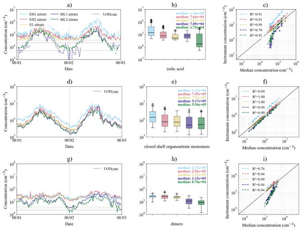
Figure 4: A great figure. A few comments. On my laptop screen the horizontal lines are hard to distinguish, so I'd recommend removing the major y-axis gridlines, which would remove two lines per panel. The caption is clear, but the figure itself could be more intuitive, especially the middle panels; I'd either label all panels (a)–(f) and clarify in the caption that the middle ones are medians calculated with different LODs, or add y-axis labels to the middle-top and middle-bottom reading "Concentration (LOD_SA)" and "Concentration (LOD_CIMS)". I'd also set the y-axis limits of the right-hand panels equal to those of the left-hand panels, so the reader can move their eye horizontally across the data. Also, the fact that the choice of LOD affects the median concentrations and the shape of the distributions so strongly is very important. Note too that the sulfuric acid concentrations rise at 08/02 00:00; this appears consistently across all instruments, and so is likely a real atmospheric phenomenon, yet occurs at concentrations well below LOD_SA, which lends further credence to LOD_SA not being the true limit of detection. Finally, I presume that in the right-hand panels the points below LOD are not included in the fits?
Figure 4: I remember an intercomparison done at the TROPOS chamber led by Peter Mettke showing that a lot of the instrument-to-instrument variability was, in fact, due to dodgy calibrations, and when everyone adopted some flat calibration number, the instruments agreed better. Not sure whether that's just papering over the cracks (so to speak) but it might be worth quickly checking for the H2SO4 time series here.
Line 455: "Nice agreement" reads as slightly too casual.
Optional: it might be nice to include a correlation matrix showing the scatter of every instrument against every other, e.g. for readers interested in how the EH instruments compare specifically against the ML instruments in the SI
Line 495: The monomer signals behave super well, but this is the sum of many peaks. What is the agreement like peak by peak? It would be interesting if the individual signals disagreed while the sum did not.
Table 6: Is this the correlation of each instrument individually against the mean of all instruments? And which LOD is used for them? It's worth clarifying this in the table caption. Also, very interesting that the agreement is so poor for organic peroxy radicals and for nitrophenol. Is this due to low signals?
Line 504: It would be useful to set up what is meant by "good agreement" and so on before line 455 so you can say good agreement as a defined term.
Line 529: Text says R2=0.853, figure shows a higher number. Also, the caption of figure 6 says it uses means while others use medians. is this right, and if so, why?
Line 547: Two compounds are named (sulfuric acid and C10H16O6), not three.
Line 595: I would be a little harsher about the I- results, which are rather poor. (This is surprising!)
Conclusions: Great, but, this is somewhat of a repetition of the abstract. It may lie outside the scope of an intercomparison paper, but if you deem it appropriate, it could be worth reframing this section as a set of practical recommendations for instrument operation and intercomparability that go beyond the usual good-practice steps we already follow.
Citation: https://doi.org/10.5194/egusphere-2026-3794-RC1 - AC1: 'Reply on RC1', Cecilia Righi, 18 Sep 2026
-
RC2: 'Comment on egusphere-2026-3794', Anonymous Referee #2, 09 Aug 2026
Please find my comments in the attached .pdf.
- AC2: 'Reply on RC2', Cecilia Righi, 18 Sep 2026
Peer review completion
Journal article(s) based on this preprint
Viewed
| HTML | XML | Total | Supplement | BibTeX | EndNote | |
|---|---|---|---|---|---|---|
| 238 | 135 | 69 | 442 | 66 | 61 | 52 |
- HTML: 238
- PDF: 135
- XML: 69
- Total: 442
- Supplement: 66
- BibTeX: 61
- EndNote: 52
Viewed (geographical distribution)
| Country | # | Views | % |
|---|
| Total: | 0 |
| HTML: | 0 |
| PDF: | 0 |
| XML: | 0 |
- 1

Mihai Ciobanu
Neha Deot
Tuija Jokinen
Chengfeng Liu
Qi Yuan
Lauriane Lucie Josette Quéléver
Spiro Jorga
Veronika Pospisilova
Lisa Beck
Mario Simon
Marcel Zauner-Wieczorek
Ruben Soler
Teresa Vera
Amalia Muñoz
Lauri Reino Ahonen
Tuukka Petäjä
The requested preprint has a corresponding peer-reviewed final revised paper. You are encouraged to refer to the final revised version.
- Preprint
(2061 KB) - Metadata XML
-
Supplement
(1768 KB) - BibTeX
- EndNote
- Final revised paper
This paper presents an intercomparison of CIMS instruments at SMEAR II. The results show variable intercomparability between CIMS instruments , where the same sulfuric acid calibration is carried over. This is unsurprising. More surprisingly, the situation for bromide is substantially better, adding further evidence that it is a good reagent ion to use. This is an extremely useful paper that addresses a real gap in knowledge for CIMS users, contains a wealth of knowledge and useful data, and I recommend it for publication. A few minor comments are provided below.
Specific comments
Line 40: "studies indicate that neutral new particle formation (NPF) dominates over ion-induced pathways in the continental boundary layer (Kerminen et al., 2010)". I believe this is true, but it may be worth referencing more recent results (e.g. Zhang et al., https://doi.org/10.1038/s41586-024-07547-1), which would support the statement across a wider range of mechanisms.
Line 53: I'd suggest a different word to "numerous", which could be read as meaning high in concentration and so contradict point (1), where the species are described as being at low concentration. Also "low in concentration" is a bit nebulous.
Line 53: The species span not only a large m/z range, functional groups and degrees of oxidation, but also a large range of carbon number, which is worth adding.
Line 73: "the operator can alter the fragmentation...". As far as I'm aware this applies mostly to the fragmentation of clusters rather than of molecules, so it might be worth specifying this.
Table 1: CEAM is not defined.
Line 122: The SI reference should point to the specific SI figure (here & throughout)
Line 145: "CI-Fi1" should read "CI-FI1" (capital I).
Line 185: It would be nice to quote the mass resolution of each instrument, perhaps the resolution at 201 m/Q (for nitrate) for nitrophenol.
Line 200: By "performance" do you mean sensitivity? And is this necessarily true, given the results of Hyttinen? the binding energies do scale linearly, but that doesn't necessarily translate to performance or sensitivity once a threshold is passed where one collision = one cluster
Line 225: It would be nice to have a brief justification for why the less-oxygenated species (e.g. C10H16O4,5,6) weren't intercompared for nitrate, since these measurements ARE sometimes used for those of us who can't run multiple chemistries simultaneously, and intercomparability would likely be even worse for these, which would be bad news.
Line 237: CI-APi-ToF is used without introduction. A sentence above might help, e.g. "APi-ToF refers to the atmospheric pressure instruments without ionisation; CI-APi-ToF to those with ionisation; CIMS is the more common parlance, as it generally also includes instruments that do not operate at atmospheric pressure."
Lines 265–268: the assumption that all the small acid peaks sit in sulfuric acid's mass range and therefore get Ctrans = 1 I think might need some consideration; iodic acid, nitrophenol, MSA and malonic acid go a fair bit higher in m/z than 97, especially HIO3NO3-, and given how steeply the transmission curves move, blanket-assigning unity to all of them could introduce a systematic bias. This might even contribute to the poor-to-moderate HA agreement in Table 6, so it's worth at least acknowledging (but probably not worth re-doing any analyses)
Line 310: A HEPA filter was used by Häkkinen, but that was in front of a VIA. It would be good to explain why it works here. I presume it's the huge surface area essentially scavenging all of the H2SO4 and HOM? A quick SI figure showing the signals going to zero with the filter in place would be helpful. Does it also work for malonic acid and other compounds? I remember seeing this done before, but not with a HEPA filter, and the signals nosedived, but didn't go to total zero.
Line 320: The CIMS LOD does indeed depend on electronic noise, but for many species it also depends on the height of an adjacent peak. For example, if quantifying iodous acid with a large HOM sitting right next to it, the tail of the HOM can swamp the iodous acid, so the LOD is a little more complex than described. I don't think this needs explicit treatment here, but it might be worth raising as a caveat of atmospheric mass spectrometry. (Optional.)
Line 327: "AIM" should be capitalised.
Line 345: Building on the earlier comment, these LODs seem very high, so it would help to back this up with the SI figure showing signals going to zero. Since the CIMS essentially operates as an ion counter, the LOD is also very sensitive to the averaging time, so this discussion could use more nuance. We also tend to be able to get sensible-looking time series below 1e5 (for example, h2so4 signals decreasing towards 1e4 as the sun goes down and rising back above 1e5 as it comes up again, which gives credence to these LODs being high).
Line 355: Very useful point. We tend to set and forget our calibrations, and this is good reason not to.
Figure 2: The spread of the data is very wide, and some points sit very far from the curve. I understand this is normal, but would it be possible to offer some practical recommendations for obtaining these curves as cleanly as possible?
Section 3.3: There is a reference error that should point to Fig. 4 (here and throughout).
Line 439: I agree it's wise to exclude the AB instrument from this figure. Would it be possible to show the H2SO4 signal time series from AB in the supplement, though? It might be useful for those of us interested in that instrument. (also totally optional)
Figure 4: A great figure. A few comments. On my laptop screen the horizontal lines are hard to distinguish, so I'd recommend removing the major y-axis gridlines, which would remove two lines per panel. The caption is clear, but the figure itself could be more intuitive, especially the middle panels; I'd either label all panels (a)–(f) and clarify in the caption that the middle ones are medians calculated with different LODs, or add y-axis labels to the middle-top and middle-bottom reading "Concentration (LOD_SA)" and "Concentration (LOD_CIMS)". I'd also set the y-axis limits of the right-hand panels equal to those of the left-hand panels, so the reader can move their eye horizontally across the data. Also, the fact that the choice of LOD affects the median concentrations and the shape of the distributions so strongly is very important. Note too that the sulfuric acid concentrations rise at 08/02 00:00; this appears consistently across all instruments, and so is likely a real atmospheric phenomenon, yet occurs at concentrations well below LOD_SA, which lends further credence to LOD_SA not being the true limit of detection. Finally, I presume that in the right-hand panels the points below LOD are not included in the fits?
Figure 4: I remember an intercomparison done at the TROPOS chamber led by Peter Mettke showing that a lot of the instrument-to-instrument variability was, in fact, due to dodgy calibrations, and when everyone adopted some flat calibration number, the instruments agreed better. Not sure whether that's just papering over the cracks (so to speak) but it might be worth quickly checking for the H2SO4 time series here.
Line 455: "Nice agreement" reads as slightly too casual.
Optional: it might be nice to include a correlation matrix showing the scatter of every instrument against every other, e.g. for readers interested in how the EH instruments compare specifically against the ML instruments in the SI
Line 495: The monomer signals behave super well, but this is the sum of many peaks. What is the agreement like peak by peak? It would be interesting if the individual signals disagreed while the sum did not.
Table 6: Is this the correlation of each instrument individually against the mean of all instruments? And which LOD is used for them? It's worth clarifying this in the table caption. Also, very interesting that the agreement is so poor for organic peroxy radicals and for nitrophenol. Is this due to low signals?
Line 504: It would be useful to set up what is meant by "good agreement" and so on before line 455 so you can say good agreement as a defined term.
Line 529: Text says R2=0.853, figure shows a higher number. Also, the caption of figure 6 says it uses means while others use medians. is this right, and if so, why?
Line 547: Two compounds are named (sulfuric acid and C10H16O6), not three.
Line 595: I would be a little harsher about the I- results, which are rather poor. (This is surprising!)
Conclusions: Great, but, this is somewhat of a repetition of the abstract. It may lie outside the scope of an intercomparison paper, but if you deem it appropriate, it could be worth reframing this section as a set of practical recommendations for instrument operation and intercomparability that go beyond the usual good-practice steps we already follow.