
the Creative Commons Attribution 4.0 License.
the Creative Commons Attribution 4.0 License.
 | 16 Jun 2026
Efficient ensemble estimation using an MCMC sampler: a reconstruction of the Mediterranean low-frequency variability combining observed and simulated sea level
Abstract. The skill of climate projections depends on the ability of models to reproduce the long-term and low-frequency variability of the system. It is thus important that low-frequency model statistics can be checked against observations. In this paper, a method is proposed to estimate directly the low-frequency component of the ocean variability from native observations using statistics from a prior long-term simulation. It is designed to account for possible model biases and to provide an estimate of the correction required to fit observations. The result is obtained by an MCMC sampler (modified to include localization of the model covariance), which provides an ensemble description of the solution, so that uncertainties can be properly assessed using independent data. This algorithm is shown well suited to work with MPI and GPUs, and efficient enough to solve large-size problems (about 108 variables and 107 observations). The approach is illustrated by the reconstruction of the low-frequency variability of the Mediterranean sea level, using statistics from a 1/12° resolution ensemble model simulation. The resulting ensemble is assessed against independent observations (by cross-validation), showing good reliability (flat rank histogram). The method also produces a consistent estimate of the model bias and of the observation error variance (mainly representativity error), while the missing prior ensemble variance is shown to be less controlable by the observations, and thus rather computed as a diagnostic. Overall, this application shows the importance of reliable model statistics, and thus the importance of enhancing model simulations to represent all main sources of uncertainty.
-
Notice on discussion status
The requested preprint has a corresponding peer-reviewed final revised paper. You are encouraged to refer to the final revised version.
-
Preprint
(6201 KB)
-
The requested preprint has a corresponding peer-reviewed final revised paper. You are encouraged to refer to the final revised version.
- Preprint
(6201 KB) - Metadata XML
- BibTeX
- EndNote
- Final revised paper


Journal article(s) based on this preprint
Interactive discussion
Status: closed
-
RC1: 'Comment on egusphere-2026-3237', Alexander Barth, 31 Jul 2026
The authors describe a novel method to deduce sea level over the Mediterranean Sea from altimetry observations and from the model results, accounting for model deficiencies in terms of bias and underestimated ensemble spread.
I think that the authors provide important results and the application here will in future lead to future improvement in the context of data assimilation. The problem that the authors address belongs to the wide class of inverse problems (including for instance also data assimilation).
In this context, virtually all approaches assume that the error covariance is perfectly known, bias free and Gaussian distributed. Which leads to a quadratic cost function which can be minimized in closed-form by solving a linear system. The paper illustrates the issue very well that when the error covariances and biases are themselves considered unknowns, closed-form solutions (e.g. Kalman Filter) are no longer available, the problem must be solved using more general techniques like the MCMC solver.
I think this paper is very well suited for Ocean Science because it includes significant theoretical advances but at the same time provides a concrete application for SSH estimation from observation and model results. They also include a description of the MCMC algorithm in the appendix to make their approach easily understandable for a wide audience.
The authors also show limitations of the initial procedure (difficulty for the convergence of the adjustment factors) and the use of additional constraints is discussed and tested.
One might question if the application of this method has not been done on a (borderline unrealistic?) hard test case where the model simulation did not include any perturbation from the forcing fields and boundary conditions and thus significantly underestimate the error variance. The method had thus to rely significantly on the adjustment of the priori error covariance. Apparently the model ensemble was not created with the purpose of providing a realistic error variance. However, if the method works with a significantly underestimated error variance it will also work for a moderate underestimation when the underlying ensemble is more realistic.
This manuscript is very well written and any question that I had while reading it was answered in the subsequent paragraph. Therefore I recommend publication with minor clarification listed here below.
Minor comment:
Line 107: ...subsequently driven by the same surface and lateral fluxes throughout the 39-year integration period (from January 1979 to December 2020). Ensemble dispersion is generated by tiny perturbations of the initial condition (as explained by Héron et al., 2026), so that the spread of the ensemble results only from the intrinsic variability of the nonlinear system
Can you comment on the lack of variability due to uncertainty in the surface fluxes?
Line 196: For future studies, could the parameter l_3, l_loc , tau_loc also be a random variable to reflect their uncertainty?
Equation 11: it seems that log and ln are both the natural logarithm. I would suggest making the notation uniform.
Line 272: For instance, with m = 30 and 6 Schur products, the number of different directions of perturbation is: N = 30×29×28×27×26×25×24 ≃ 1.026×10^10 , which is sufficient to span all relevant degrees of freedom of our system.
The fact that here m=30 is it related to choice of the number of ensemble members which is also 30r? It seems that these two are unrelated, or not? The number of directions is substantial, but their usefulness also depends on how the initial perturbations are chosen? Can you give more details on this? Would a rough lower bound be the area (or volume) of the domain divided by the effective support of the localization function, adjusted by the sqrt(6) parameter? (by effective support I mean, loosely speaking, the area where localization function is significantly different from nonzero)
Line 305: From Fig. fig:map:posterior…: The figure number is missing
Citation: https://doi.org/10.5194/egusphere-2026-3237-RC1 -
AC1: 'Reply on RC1', Jean-Michel Brankart, 28 Sep 2026
We thank the reviewer for his careful reading of the manuscript and for his appreciation of the work done in this study. Please find below a detailed answer to all comments.
- Yes, it is true that the ensemble was not produced specifically for this study. Important sources of uncertainties (e.g. in the atmospheric forcing and in the boundary conditions) were not taken into account; this is why we could not rely on the prior variance (basically we only use the local correlation structure), and why an adjustment of the ensemble statistics is even more important. In any case, it is difficult to produce model ensembles with an appropriate spread, which is why an adjustment procedure is useful. This difficulty was already emphasized in the last paragraph of the conclusions, but it is true that this should be done before that.
We have thus added the following sentences in section 2.2 (line 119) to warn the reader about this from the very beginning: "This ensemble was indeed not specifically produced for this paper, but was dedicated to the specific study of intrinsic variability by Héron et al. (2026). Important sources of uncertainties (e.g. in the atmospheric forcing and in the boundary conditions) were not taken into account; this is why we could not rely on the prior variance, and why an adjustment of the ensemble statistics is even more important."
- In principle, yes, any parameter could be included in the estimation vector. But, with our method, this is not true for the parameters controlling the covariance localization (l_3, l_loc,, tau_loc), because the ensemble of vectors with correlation given by Eq. (13), which depends on these parameters, and which are used to compute perturbations with the right localized covariance, must be computed once and for all before the MCMC iterations.
- Yes, we have made the notation uniform, i.e. "log" to mean the natural logarithm.
- Yes, the effective number of degrees of freedom (d) in our system is much smaller than N, and it indeed depends on the ratio between the size of the domain (in space and time) and the localization scales. Moreover, only a tiny fraction of the N possibilities for the perturbations are effectively used in the iterations. However, if we want to produce a quasi-random sample in a space of dimension d, it is always good if the number of directions of perturbation N (which is here discrete because of the finite sample) can be very large.
On the other hand, yes, it is also true that the size of the ensemble of vectors that are used for the localization of the prior ensemble [with correlation given by Eq. (13)] does not need to be the same as the size of the prior ensemble itself. It would be quite easy to use a larger sample (with just more memory), and this could make N even larger. We have used the same size here because it is technically more simple if the two ensembles have the same size, and to limit the memory requirements. It can also be noted that this "localizing ensemble" was originally intended to be a smoother version of the original ensemble and had thus the same size by construction (see Brankart, 2019).
This has been clarified by adding the following sentences in section 3.4 (line 273): "Actually, the effective number of degrees of freedom (d) depends on the ratio between the size of the domain (in space and time) and the localization scales, and it is very tiny as compared to N. The idea behind this large value of N is to produce a quasi-random sample of this target space of dimension d, and thus ideally among the largest possible number of directions of perturbation (which has here to be discrete because of the finite samples). See Brankart (2019) for more details. It must also be mentioned that the size of the localizing ensemble could also be larger than the size of the original ensemble, which would also increase N. We used here the same size for simplicity and to limit the memory requirements."
Citation: https://doi.org/10.5194/egusphere-2026-3237-AC1
-
AC1: 'Reply on RC1', Jean-Michel Brankart, 28 Sep 2026
-
RC2: 'Comment on egusphere-2026-3237', Benedicte Lemieux-Dudon, 09 Sep 2026
The authors propose an original ensemble-based approach designed to improve the representation of the long-term and low-frequency variability of the climate system (ocean compart)by providing an appropriate probabilistic initial condition for carrying out climate projections.
The authors formulate a Bayesian inverse problem in which the main unknown is the Sea Surface Height (SSH) in the Mediterranean Sea (MED) and where the objective is to reconstruct the interannual SSH variability between 1995 and 2019 by using along-track satellite altimetry observations to constrain the problem. For that purpose by using the NEMO hydrodynamic model, the authors construct a prior ensemble of simulations ( 30-members ) by perturbing the only initial condition, after a one-member spin-up period to asses the prior probability distribution (pdf) of the inverse problem. The prior pdf is mainly described by the ensemble mean and error covariance matrix. To reduce the sampling errors related to the limited size of the ensemble, the correlation of the prior ensemble members are localized in space and time using a Schur product involving Gaussian kernels. The authors introduce additional statistical parameters in the control vector. These parameters are also identified along with the low-frequency SSH time evolution. The existence of a prior ensemble bias motivates the authors to also control stationary in time biases in the Dynamic Height, Temperature and Salinity fields. Also, the spread of the prior ensemble being insufficient to explain the misfit with observations, the authors decide to also control the error variance both on the prior SSH estimate and the satellite altimetry observations. Due to these auxiliary statistical parameters introduced to control the bias and the spread, the overall prior probability distribution becomes non-gaussian. According to the Bayesian framework, the authors combine the prior probability distribution with the likelihood based on the altimetry observations and derive a cost function which is non-quadratic since the problem is non-linear. They propose to apply a Markov Chain Monte Carlo solver (MCMC) to sample the posterior probability distribution, rejecting or accepting the Markov Chain candidate iterate based on the increase or decrease of the cost function. This MCMC method applies a variant of the Metropolis/Hastings algorithm : the drawing of the random direction of perturbation to construct the Markov Chain candidate iterate involves the use of Schur products designed in such a way that the covariance of the pseudo-random direction of perturbation is the covariance of the localized prior ensemble. With such a variant, the MCMC rejection/acceptance of the candidate iterate is only driven by the likelihood function.
At the end, the method enables to obtain an updated ensemble with members sampling the posterior probability function with a posterior estimate of the Dynamic Height evolution in the MED sea. The authors discuss their results and propose different approaches to validate the Dynamic Height reconstruction.
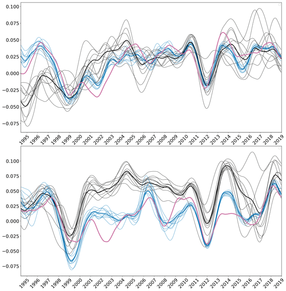
First, they compare the interannual variability of the reconstructed Dynamic Height maps to the AVISO L4 product : compared to the prior ensemble, the spread of the posterior ensemble appears to be reduced at time period and location where dense along-track altimetry measurements are available. The authors also propose a cross-validation framework using part of the observations to constrain the likelihood and keeping the other part for validation. In this manner, they can assess the reliability of the updated ensemble by using rank-histogram with independent observations. They discuss the reconstructed Dynamic Height bias as well as the updated ensemble spread and tuned observation error variance.
The article is very well written. The authors provide many details so that the reader can understand the chosen methodology. The authors tackle a complicated estimation problem with non-gaussian distributions, biased datasets and ensemble spread issues. Outside the Gaussian and linear context, solving inverse problems is a challenging task. They apply an original variant of the MCMC Metropolis/Hastings algorithm which enables to optimize the MCMC solver, re-using the ensemble localization operator. They test this algorithm on a realistic application, which contributes to methodological progress.
I recommend the publication of this article. I have only few minor comments/questions that are listed below.
Minor comments/questions :
- L30 simulationsimulationss -> simulations
- Eqn 8 : gamma_loc depends on r and delta_t, for the sake of clarity I suggest you had the delta_t dependence on the LHS of the equation.
- L183 + Eqn 5, L215 + Eqn 10 : you decide to tune the prior ensemble error variance (Pr,1 matrix with the alpha diagonal matrix) because the spread of the ensemble is not sufficient to explain the misfit with altimetry observations. Why also tuning the observation error variance (Rr matrix with the beta diagonal matrix) ? You explain that it should account for the observation representativity error. Could the tuning of both alpha and beta vectors lead to introduce unnecessary degrees of freedom in the inverse problem ? Can this affect the MCMC convergence ? Regarding the alpha parameter (spread) ?
- Eqn 11 : in the quest for accuracy, I would suggest adding a constant value to the LHS of the cost function observation term, so that equality between the LHS and RHS of equation 11 holds, even if at the "minimization" stage this extra constant term won't play any role.
- In the discussion, you did not comment on the Temperature or Salinity biases reconstruction. Are those two biases consistent with the Dynamic Height bias ?
- To produce the prior ensemble, can you explain further why you choose to only perturb the initial condition ?
- Figure 5 : for the reliability diagrams, I would suggest using the same scale for the Y-axis of the top pannel plots on one hand, and also for bottom pannel plots on the other hand. This way we would clearly see (top pannel) that SSH-B experiment assimilates more observations than the SSH-A experiment. For the bottom pannel we expect the same amount of verifying observations for the two rank histograms. Could this help to compare the distorsion of the reliability in a more quantitative manner ?
Citation: https://doi.org/10.5194/egusphere-2026-3237-RC2 -
AC2: 'Reply on RC2', Jean-Michel Brankart, 28 Sep 2026
We thank the reviewer for her careful reading of the manuscript and for her appreciation of the work done in this study. Please find below a detailed answer to all comments.
- The typo has been fixed.
- Yes, it is indeed much better to make the dependence in Delta_t explicit in the LHS. This has been corrected.
- Yes, indeed. This can be a source of problem and can affect the convergence of the Markov chains. In principle, the two factors can be estimated simultaneously if prior uncertainties and observation uncertainties have distinct correlation structures and if there are enough observations (as in adaptive Kalman filters). But the non-convergence of alpha in the results means that information is missing. Maybe adding an additional constraint on alpha would be necessary to control correctly the two parameters.
It is indeed useful to add a caution about this already in section 3.1. We have added the following text: "It must be noted here that it may be challenging to estimate these two factors simultaneously, since it is always the sum of the prior and observation uncertainties that is observed. The joint estimate is still possible in principle (as in adaptive Kalman filters) if they have distinct correlation structures, but it is always possible that information is missing to obtain accurate estimates."
- Yes, indeed, there is a constant missing in Eq. (11). It has been added.
- This paper is only focused on dynamic height. There are also biases in the model temperature and salinity. Part of them are related to dynamic height. Others are not. We made preliminary attempts (not included in the paper) to work on the multivariate problem, but biases are more difficult to identify in this case, because of the ever changing coverage of temperature and salinity observations.
- Yes, this is related to a question raised by Reviewer 1. This is because the ensemble was not produced specifically for this study, but for the paper by Héron et al. (2026), which was dedicated to the study of the intrinsic variability whose emergence is triggered by initial condition perturbations.
The following sentences has been added in section 2.2 (line 119) to clarify this point: "This ensemble was indeed not specifically produced for this paper, but was dedicated to the specific study of intrinsic variability by Héron et al. (2026). Important sources of uncertainties (e.g. in the atmospheric forcing and in the boundary conditions) were not taken into account; this is why we could not rely on the prior variance, and why an adjustment of the ensemble statistics is even more important."
- Regarding the top panels Fig. 5, yes, it would have been an option to keep the same scale for the Y-axis. But what matters here is more to compare the shape of the histograms, which would be less obvious is we adjust the scales. The total number of observations is more like a secondary information here, which is even often dropped by normalizing the histograms.
Regarding the bottom panels of Fig. 5, yes, indeed, the total amount of verifying variables must be the same in the two panels. The integral of the two histograms is the same. In this case, it is indeed much better if we use the same scale for the Y-axis. The two panels have been redrawn to correct this. The close similarity between the two histograms is now more clearly visible. Only the external maxima are notably different.
Citation: https://doi.org/10.5194/egusphere-2026-3237-AC2
Peer review completion


Interactive discussion
Status: closed
-
RC1: 'Comment on egusphere-2026-3237', Alexander Barth, 31 Jul 2026
The authors describe a novel method to deduce sea level over the Mediterranean Sea from altimetry observations and from the model results, accounting for model deficiencies in terms of bias and underestimated ensemble spread.
I think that the authors provide important results and the application here will in future lead to future improvement in the context of data assimilation. The problem that the authors address belongs to the wide class of inverse problems (including for instance also data assimilation).
In this context, virtually all approaches assume that the error covariance is perfectly known, bias free and Gaussian distributed. Which leads to a quadratic cost function which can be minimized in closed-form by solving a linear system. The paper illustrates the issue very well that when the error covariances and biases are themselves considered unknowns, closed-form solutions (e.g. Kalman Filter) are no longer available, the problem must be solved using more general techniques like the MCMC solver.
I think this paper is very well suited for Ocean Science because it includes significant theoretical advances but at the same time provides a concrete application for SSH estimation from observation and model results. They also include a description of the MCMC algorithm in the appendix to make their approach easily understandable for a wide audience.
The authors also show limitations of the initial procedure (difficulty for the convergence of the adjustment factors) and the use of additional constraints is discussed and tested.
One might question if the application of this method has not been done on a (borderline unrealistic?) hard test case where the model simulation did not include any perturbation from the forcing fields and boundary conditions and thus significantly underestimate the error variance. The method had thus to rely significantly on the adjustment of the priori error covariance. Apparently the model ensemble was not created with the purpose of providing a realistic error variance. However, if the method works with a significantly underestimated error variance it will also work for a moderate underestimation when the underlying ensemble is more realistic.
This manuscript is very well written and any question that I had while reading it was answered in the subsequent paragraph. Therefore I recommend publication with minor clarification listed here below.
Minor comment:
Line 107: ...subsequently driven by the same surface and lateral fluxes throughout the 39-year integration period (from January 1979 to December 2020). Ensemble dispersion is generated by tiny perturbations of the initial condition (as explained by Héron et al., 2026), so that the spread of the ensemble results only from the intrinsic variability of the nonlinear system
Can you comment on the lack of variability due to uncertainty in the surface fluxes?
Line 196: For future studies, could the parameter l_3, l_loc , tau_loc also be a random variable to reflect their uncertainty?
Equation 11: it seems that log and ln are both the natural logarithm. I would suggest making the notation uniform.
Line 272: For instance, with m = 30 and 6 Schur products, the number of different directions of perturbation is: N = 30×29×28×27×26×25×24 ≃ 1.026×10^10 , which is sufficient to span all relevant degrees of freedom of our system.
The fact that here m=30 is it related to choice of the number of ensemble members which is also 30r? It seems that these two are unrelated, or not? The number of directions is substantial, but their usefulness also depends on how the initial perturbations are chosen? Can you give more details on this? Would a rough lower bound be the area (or volume) of the domain divided by the effective support of the localization function, adjusted by the sqrt(6) parameter? (by effective support I mean, loosely speaking, the area where localization function is significantly different from nonzero)
Line 305: From Fig. fig:map:posterior…: The figure number is missing
Citation: https://doi.org/10.5194/egusphere-2026-3237-RC1 -
AC1: 'Reply on RC1', Jean-Michel Brankart, 28 Sep 2026
We thank the reviewer for his careful reading of the manuscript and for his appreciation of the work done in this study. Please find below a detailed answer to all comments.
- Yes, it is true that the ensemble was not produced specifically for this study. Important sources of uncertainties (e.g. in the atmospheric forcing and in the boundary conditions) were not taken into account; this is why we could not rely on the prior variance (basically we only use the local correlation structure), and why an adjustment of the ensemble statistics is even more important. In any case, it is difficult to produce model ensembles with an appropriate spread, which is why an adjustment procedure is useful. This difficulty was already emphasized in the last paragraph of the conclusions, but it is true that this should be done before that.
We have thus added the following sentences in section 2.2 (line 119) to warn the reader about this from the very beginning: "This ensemble was indeed not specifically produced for this paper, but was dedicated to the specific study of intrinsic variability by Héron et al. (2026). Important sources of uncertainties (e.g. in the atmospheric forcing and in the boundary conditions) were not taken into account; this is why we could not rely on the prior variance, and why an adjustment of the ensemble statistics is even more important."
- In principle, yes, any parameter could be included in the estimation vector. But, with our method, this is not true for the parameters controlling the covariance localization (l_3, l_loc,, tau_loc), because the ensemble of vectors with correlation given by Eq. (13), which depends on these parameters, and which are used to compute perturbations with the right localized covariance, must be computed once and for all before the MCMC iterations.
- Yes, we have made the notation uniform, i.e. "log" to mean the natural logarithm.
- Yes, the effective number of degrees of freedom (d) in our system is much smaller than N, and it indeed depends on the ratio between the size of the domain (in space and time) and the localization scales. Moreover, only a tiny fraction of the N possibilities for the perturbations are effectively used in the iterations. However, if we want to produce a quasi-random sample in a space of dimension d, it is always good if the number of directions of perturbation N (which is here discrete because of the finite sample) can be very large.
On the other hand, yes, it is also true that the size of the ensemble of vectors that are used for the localization of the prior ensemble [with correlation given by Eq. (13)] does not need to be the same as the size of the prior ensemble itself. It would be quite easy to use a larger sample (with just more memory), and this could make N even larger. We have used the same size here because it is technically more simple if the two ensembles have the same size, and to limit the memory requirements. It can also be noted that this "localizing ensemble" was originally intended to be a smoother version of the original ensemble and had thus the same size by construction (see Brankart, 2019).
This has been clarified by adding the following sentences in section 3.4 (line 273): "Actually, the effective number of degrees of freedom (d) depends on the ratio between the size of the domain (in space and time) and the localization scales, and it is very tiny as compared to N. The idea behind this large value of N is to produce a quasi-random sample of this target space of dimension d, and thus ideally among the largest possible number of directions of perturbation (which has here to be discrete because of the finite samples). See Brankart (2019) for more details. It must also be mentioned that the size of the localizing ensemble could also be larger than the size of the original ensemble, which would also increase N. We used here the same size for simplicity and to limit the memory requirements."
Citation: https://doi.org/10.5194/egusphere-2026-3237-AC1
-
AC1: 'Reply on RC1', Jean-Michel Brankart, 28 Sep 2026
-
RC2: 'Comment on egusphere-2026-3237', Benedicte Lemieux-Dudon, 09 Sep 2026
The authors propose an original ensemble-based approach designed to improve the representation of the long-term and low-frequency variability of the climate system (ocean compart)by providing an appropriate probabilistic initial condition for carrying out climate projections.
The authors formulate a Bayesian inverse problem in which the main unknown is the Sea Surface Height (SSH) in the Mediterranean Sea (MED) and where the objective is to reconstruct the interannual SSH variability between 1995 and 2019 by using along-track satellite altimetry observations to constrain the problem. For that purpose by using the NEMO hydrodynamic model, the authors construct a prior ensemble of simulations ( 30-members ) by perturbing the only initial condition, after a one-member spin-up period to asses the prior probability distribution (pdf) of the inverse problem. The prior pdf is mainly described by the ensemble mean and error covariance matrix. To reduce the sampling errors related to the limited size of the ensemble, the correlation of the prior ensemble members are localized in space and time using a Schur product involving Gaussian kernels. The authors introduce additional statistical parameters in the control vector. These parameters are also identified along with the low-frequency SSH time evolution. The existence of a prior ensemble bias motivates the authors to also control stationary in time biases in the Dynamic Height, Temperature and Salinity fields. Also, the spread of the prior ensemble being insufficient to explain the misfit with observations, the authors decide to also control the error variance both on the prior SSH estimate and the satellite altimetry observations. Due to these auxiliary statistical parameters introduced to control the bias and the spread, the overall prior probability distribution becomes non-gaussian. According to the Bayesian framework, the authors combine the prior probability distribution with the likelihood based on the altimetry observations and derive a cost function which is non-quadratic since the problem is non-linear. They propose to apply a Markov Chain Monte Carlo solver (MCMC) to sample the posterior probability distribution, rejecting or accepting the Markov Chain candidate iterate based on the increase or decrease of the cost function. This MCMC method applies a variant of the Metropolis/Hastings algorithm : the drawing of the random direction of perturbation to construct the Markov Chain candidate iterate involves the use of Schur products designed in such a way that the covariance of the pseudo-random direction of perturbation is the covariance of the localized prior ensemble. With such a variant, the MCMC rejection/acceptance of the candidate iterate is only driven by the likelihood function.
At the end, the method enables to obtain an updated ensemble with members sampling the posterior probability function with a posterior estimate of the Dynamic Height evolution in the MED sea. The authors discuss their results and propose different approaches to validate the Dynamic Height reconstruction.
First, they compare the interannual variability of the reconstructed Dynamic Height maps to the AVISO L4 product : compared to the prior ensemble, the spread of the posterior ensemble appears to be reduced at time period and location where dense along-track altimetry measurements are available. The authors also propose a cross-validation framework using part of the observations to constrain the likelihood and keeping the other part for validation. In this manner, they can assess the reliability of the updated ensemble by using rank-histogram with independent observations. They discuss the reconstructed Dynamic Height bias as well as the updated ensemble spread and tuned observation error variance.
The article is very well written. The authors provide many details so that the reader can understand the chosen methodology. The authors tackle a complicated estimation problem with non-gaussian distributions, biased datasets and ensemble spread issues. Outside the Gaussian and linear context, solving inverse problems is a challenging task. They apply an original variant of the MCMC Metropolis/Hastings algorithm which enables to optimize the MCMC solver, re-using the ensemble localization operator. They test this algorithm on a realistic application, which contributes to methodological progress.
I recommend the publication of this article. I have only few minor comments/questions that are listed below.
Minor comments/questions :
- L30 simulationsimulationss -> simulations
- Eqn 8 : gamma_loc depends on r and delta_t, for the sake of clarity I suggest you had the delta_t dependence on the LHS of the equation.
- L183 + Eqn 5, L215 + Eqn 10 : you decide to tune the prior ensemble error variance (Pr,1 matrix with the alpha diagonal matrix) because the spread of the ensemble is not sufficient to explain the misfit with altimetry observations. Why also tuning the observation error variance (Rr matrix with the beta diagonal matrix) ? You explain that it should account for the observation representativity error. Could the tuning of both alpha and beta vectors lead to introduce unnecessary degrees of freedom in the inverse problem ? Can this affect the MCMC convergence ? Regarding the alpha parameter (spread) ?
- Eqn 11 : in the quest for accuracy, I would suggest adding a constant value to the LHS of the cost function observation term, so that equality between the LHS and RHS of equation 11 holds, even if at the "minimization" stage this extra constant term won't play any role.
- In the discussion, you did not comment on the Temperature or Salinity biases reconstruction. Are those two biases consistent with the Dynamic Height bias ?
- To produce the prior ensemble, can you explain further why you choose to only perturb the initial condition ?
- Figure 5 : for the reliability diagrams, I would suggest using the same scale for the Y-axis of the top pannel plots on one hand, and also for bottom pannel plots on the other hand. This way we would clearly see (top pannel) that SSH-B experiment assimilates more observations than the SSH-A experiment. For the bottom pannel we expect the same amount of verifying observations for the two rank histograms. Could this help to compare the distorsion of the reliability in a more quantitative manner ?
Citation: https://doi.org/10.5194/egusphere-2026-3237-RC2 -
AC2: 'Reply on RC2', Jean-Michel Brankart, 28 Sep 2026
We thank the reviewer for her careful reading of the manuscript and for her appreciation of the work done in this study. Please find below a detailed answer to all comments.
- The typo has been fixed.
- Yes, it is indeed much better to make the dependence in Delta_t explicit in the LHS. This has been corrected.
- Yes, indeed. This can be a source of problem and can affect the convergence of the Markov chains. In principle, the two factors can be estimated simultaneously if prior uncertainties and observation uncertainties have distinct correlation structures and if there are enough observations (as in adaptive Kalman filters). But the non-convergence of alpha in the results means that information is missing. Maybe adding an additional constraint on alpha would be necessary to control correctly the two parameters.
It is indeed useful to add a caution about this already in section 3.1. We have added the following text: "It must be noted here that it may be challenging to estimate these two factors simultaneously, since it is always the sum of the prior and observation uncertainties that is observed. The joint estimate is still possible in principle (as in adaptive Kalman filters) if they have distinct correlation structures, but it is always possible that information is missing to obtain accurate estimates."
- Yes, indeed, there is a constant missing in Eq. (11). It has been added.
- This paper is only focused on dynamic height. There are also biases in the model temperature and salinity. Part of them are related to dynamic height. Others are not. We made preliminary attempts (not included in the paper) to work on the multivariate problem, but biases are more difficult to identify in this case, because of the ever changing coverage of temperature and salinity observations.
- Yes, this is related to a question raised by Reviewer 1. This is because the ensemble was not produced specifically for this study, but for the paper by Héron et al. (2026), which was dedicated to the study of the intrinsic variability whose emergence is triggered by initial condition perturbations.
The following sentences has been added in section 2.2 (line 119) to clarify this point: "This ensemble was indeed not specifically produced for this paper, but was dedicated to the specific study of intrinsic variability by Héron et al. (2026). Important sources of uncertainties (e.g. in the atmospheric forcing and in the boundary conditions) were not taken into account; this is why we could not rely on the prior variance, and why an adjustment of the ensemble statistics is even more important."
- Regarding the top panels Fig. 5, yes, it would have been an option to keep the same scale for the Y-axis. But what matters here is more to compare the shape of the histograms, which would be less obvious is we adjust the scales. The total number of observations is more like a secondary information here, which is even often dropped by normalizing the histograms.
Regarding the bottom panels of Fig. 5, yes, indeed, the total amount of verifying variables must be the same in the two panels. The integral of the two histograms is the same. In this case, it is indeed much better if we use the same scale for the Y-axis. The two panels have been redrawn to correct this. The close similarity between the two histograms is now more clearly visible. Only the external maxima are notably different.
Citation: https://doi.org/10.5194/egusphere-2026-3237-AC2
Peer review completion
Journal article(s) based on this preprint
Data sets
Low-frequency variability of the Mediterranean dynamic height: an ensemble estimation combining model and observations J.-M. Brankart et al. https://doi.org/10.17882/113890
Viewed
| HTML | XML | Total | BibTeX | EndNote | |
|---|---|---|---|---|---|
| 168 | 63 | 28 | 259 | 21 | 17 |
- HTML: 168
- PDF: 63
- XML: 28
- Total: 259
- BibTeX: 21
- EndNote: 17
Viewed (geographical distribution)
| Country | # | Views | % |
|---|
| Total: | 0 |
| HTML: | 0 |
| PDF: | 0 |
| XML: | 0 |
- 1
Jean-Michel Brankart

Damien Héron
Lisa Weiss
Thierry Penduff
Pierre Brasseur
The requested preprint has a corresponding peer-reviewed final revised paper. You are encouraged to refer to the final revised version.
- Preprint
(6201 KB) - Metadata XML