
the Creative Commons Attribution 4.0 License.
the Creative Commons Attribution 4.0 License.
 | 11 Jun 2026
Quantifying Drivers of Tropospheric OH and Its Trends: Sensitivity to Atmospheric Processes and Implications for Methane Lifetime
Abstract. The hydroxyl radical (OH) is a critical determinant of global oxidative capacity and trace gas lifetimes, but its variation remains poorly constrained. This study investigates the sensitivity of modelled tropospheric OH concentration changes to physical and chemical processes using the FRSGC/UCI chemistry transport model. The simulated tropospheric O3 and NO2 agree well with satellite observations, but that annual variations in CO do not, likely due to uncertainties in biomass burning emissions in the southern hemisphere and overestimated CO trends over Asia. This discrepancy, along with the background increase in CO, may lead to an underestimation of OH increase or overestimation of OH decrease from 2000 to 2017. Changes in tropospheric OH column show substantial spatial heterogeneity, with increases in OH in high-emission regions and decreases in the tropics. Global mean OH trends are dependent on the assumed trend in emissions: with dynamic emissions there is little change in OH, while under annually invariant emissions, there is a substantial increase in OH due to meteorological conditions alone. Inclusion of water vapor UV absorption, heterogeneous reactions, and updates to the OH + NO2 reaction rate have a smaller impact on OH trend, but decrease OH levels by 3.6%, 5.8%, and 7.0%, respectively, increasing CH4 lifetimes by 4.2%, 5.2%, and 8.4%. Incorporating oceanic CH3CHO emissions reduces global mean OH by up to 1.5%, increasing the CH4 lifetime by up to 1.6%. These results provide a quantitative basis for understanding the drivers of tropospheric OH variability and their implications for global methane chemistry.
Competing interests: At least one of the (co-)authors is a member of the editorial board of Atmospheric Chemistry and Physics.
Publisher's note: Copernicus Publications remains neutral with regard to jurisdictional claims made in the text, published maps, institutional affiliations, or any other geographical representation in this paper. While Copernicus Publications makes every effort to include appropriate place names, the final responsibility lies with the authors. Views expressed in the text are those of the authors and do not necessarily reflect the views of the publisher.-
Notice on discussion status
The requested preprint has a corresponding peer-reviewed final revised paper. You are encouraged to refer to the final revised version.
-
Preprint
(3797 KB)
-
Supplement
(1333 KB)
-
The requested preprint has a corresponding peer-reviewed final revised paper. You are encouraged to refer to the final revised version.
- Preprint
(3797 KB) - Metadata XML
-
Supplement
(1333 KB) - BibTeX
- EndNote
- Final revised paper


Journal article(s) based on this preprint
Interactive discussion
Status: closed
-
CC1: 'Data Provider Acknowledgement', Glenn Wolfe, 11 Jun 2026
-
AC1: 'Reply on CC1', Xuewei Hou, 11 Jun 2026
Many apologies for this oversight. We will be sure to add an acknowledgment in any revised manuscript.
Citation: https://doi.org/10.5194/egusphere-2026-3114-AC1
-
AC1: 'Reply on CC1', Xuewei Hou, 11 Jun 2026
-
RC1: 'Comment on egusphere-2026-3114', Anonymous Referee #1, 02 Jul 2026
This paper investigates the sensitivity of the global OH and its trends simulated by a chemistry transport model to processes including water vapor UV absorption, heterogeneous reactions, the OH + NO2 reaction rate, and oceanic CH3CHO emissions. The model is validated against observations of multiple species. Understanding the drivers of OH concentrations and changes is an important topic. An overestimate of global mean OH is a common feature of global models, so quantifying the impact of these processes on the simulated OH is of strong interest. The methods are generally robust, but some clarifications of the methodology and conclusions are needed, as described in the comments below.
General Comments:
1. The introduction provides a nice overview of the recent developments related to modeling processes relevant to OH. However, it would benefit from a clearer articulation of what the open questions related to these processes are that this paper seeks to address. The conclusions could be strengthened by putting the results in the context of the open questions. In particular, the conclusions give a summary of how each of the individual processes impact OH levels in the model, but I think the paper would have more impact if it can tie that information back to the motivating issues raised in the introduction. For example, would including all these processes be expected to resolve all (or a fraction) of the OH bias seen in model intercomparisons?
2. The introduction motivates the study in part by highlighting the tendency of global models to overestimate global OH and underestimate methane lifetime. However, the manuscript also states on line 608 that “Airmass-weighted OH concentrations and methane lifetimes in this study are fully consistent with observational and multi-model estimates”, which suggests this bias is not present in the model used in this study. Is it the incorporation of the new processes/rates that allows the model to be consistent with observational estimates? If so, please clarify this.
3. While the control run includes most of the processes considered in the study and the effects of the processes are quantified by removing the process in a sensitivity run, the impact of oceanic CH3CHO emissions seems to be quantified in the opposite way, e.g. included in a sensitivity run but not the control. A couple sentences clarifying and justifying this distinction would be helpful. See also specific comment 4.
Specific Comments:
- Line 71: I don’t understand the statement “NOx chemistry extended the model estimate…”. Does it mean the model estimate increased?
- Line 167: Why is a climatology used for the aerosols? Since the paper aims to quantify the impact of heterogeneous chemistry on OH trends, it would be preferable to include interannual variability in the aerosols.
- Line 182: What lightning parameterization is used?
- Line 192: Related to general comment 2, the text here states that the control run includes all the processes detailed above. However, it later appears that the control run does not include ocean emissions of CH3CHO. Please clarify.
- Section 3 contains a lot of general model evaluation. I recommend focusing the discussion on the implications of the evaluation for OH. A summary table might be helpful.
- Line 288: Is this the correlation of the timeseries of annual mean modeled O3 with OMI/MLS O3 at each grid box?
- Line 293: Could mismatches between modeled and OMI/MLS tropopause be involved?
- Line 294: How is the seasonal cycle involved? I thought the correlations were for the annual mean. Please clarify.
- Lines 316-318: The text states “Overall, our simulated results represent the distributions and interannual variations of O3 well”, but Fig. 1e,f shows substantial differences between the modeled and OMI/MLS tropospheric O3 column trends. This could potentially impact simulated OH trends.
- Section 3.1-3.2: It might make sense to either reorder the discussion of section 3.1 to discuss O3 last, or else move section 3.2 before section 3.1, to put the discussion of satellite O3 next to the discussion of surface O3.
- Table 3: Some of the differences in [OH]gm between simulations are pretty small. Could you add the range of [OH]gm for individual years or else the standard deviation over all years so that the difference between simulations can be compared to the magnitude of year-to-year variability?
- Line 469: Can this result be shown on Fig. 5?
- Line 532 and Fig. 9: Can the color scale of the figure be extended so that it doesn’t max out over such a large region of Asia? Also, what explains the location of the OH maximum in the annual mean? Is it related to the terrain?
- Section 4.4 last paragraph: How do these trend results compare to those of Souri et al., 2024 (https://doi.org/10.5194/acp-24-8677-2024)?
- Line 547: This would be a good place to also mention the possible effects of the model mismatches with the OMI/MLS O3 trend.
- Table 6: Can you add the uncertainty in the trends to the table? This would help show how statistically different the trends in the different simulations are from each other.
- Line 562-563: Can you say which meteorological differences drive the trend?
- Fig. 10: Does “Mete” in the legend correspond to the fixed emission run? If so, please clarify this in the caption.
- Line 581: The statement “effectively reduce this overestimation without substantially altering the OH trend, thereby improving model performance” seems to imply that not altering the OH trend is important to preserving model performance. But do we know the model OH trend is correct?
- Line 583-584: Why does heterogeneous chemistry on clouds suppress the trend? Is there a trend in the model clouds?
- Line 584: Isn’t the little influence of aerosols on the OH interannual variability expected from the use of climatological aerosols? Accurately quantifying this effect on interannual variability would require including aerosol interannual variability in the simulation.
- Line 255-257: Explain how changing a reaction that contributes only 1% of OH loss changes the global mean OH by 7%.
- Last paragraph of Section 4: This paragraph would be stronger if it highlighted what new insights into the OH variations are obtained from this comparison. If this comparison is more for model validation, then I recommend moving it further up in the text.
- Last 2 sentences: Can you add something more specific about which processes most need improved representation? Also, does improving representation in this context mean further research to understand the processes, or incorporating the current understanding of the processes into more models?
- Supplement Fig. S6: I couldn’t find a reference to this figure in the text. How does it differ from the right side of Fig. 9?
- Some papers listed in the references do not appear to be cited in the text.
Citation: https://doi.org/10.5194/egusphere-2026-3114-RC1 - AC2: 'Reply on RC1', Xuewei Hou, 21 Aug 2026
-
RC2: 'Comment on egusphere-2026-3114', Anonymous Referee #2, 07 Jul 2026
Hou et al. present an evaluation of OH trends from year 2000 to 2017 using a chemistry transport model and their drivers. The studies includes a thorough evaluation of the model with observations. Another novelty of the study is the exploration of the role of introducing newer atmospheric processes, updated rate constants and new oceanic emissions on OH and methane lifetime. The paper is generally well-written, highly relevant to the scope of ACP, and the exploration of new processes / rate constant/ emissions is extremely relevant and valuable to the modelling community. I have some comments which I hope the authors will consider, but other than that, recommend publication.
General comments:
- The authors have presented a thorough evaluation of drivers of OH, namely ozone and CO. I was wondering if the authors ever explored how the inclusion/exclusion of the different OH processes affects model performance for these drivers too? Although I understand it gets a bit circular sometimes (the drivers affect OH, but OH also potentially affects the drivers). It just may be of interest to the community to also see how the different processes suggested could affect model performance across multiple metrics.
- I have a similar question as he other anonymous reviewer: why do the authors deem that preserving the OH trend across different processes is a goal if there are uncertainties in the trend itself?
Specific comments:
Title: Not sure if it would be good to put the time period in the title? Also, a key novelty is the exploration of physical mechanisms not currently employed in most models, so I was wondering if the title could somehow reflect this? Just some suggestions to make the title more specific and also highlight novel aspects, since the title currently reads as quite general.
Abstract: ‘substantial increase in OH’: I guess I’m not really certain what would constitute as a ‘substantial’ increase? Also,‘dynamic emissions’ - would suggest rewording this to say ‘time-varying emissions’?
Line 39: The authors mention ‘future atmospheric composition’, whereas the studies cited (Stevenson 2020, Lelieveld 2016, Chua 2023) are historical. Perhaps some studies like Voulgarakis et al. (2013), Liu et al. (2024) or Chua et al. (2026) could be useful as some examples of future scenario OH / methane lifetime drivers, though I guess if the broader point is about exploring the ‘interactions between natural and anthropogenic emissions and climate change’, then it could be fine to remain as is.
Introduction:
Table 4: Why is there a table entry that is bolded?
Line 270: Would suggest not using the term ‘long-term’ for the study period of 17 years.
Line 275: ‘airmass’ rather than mass?
Figure 7:
- Panel (a) title units should say ‘molec cm-3’ not ‘moles cm-3’.
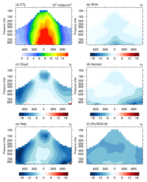
- Currently, the caption which says ‘difference in OH (in %) in the troposphere due to (b) removing water vapour UV absorption (WVA) …’., but perhaps it would be helpful for the reader to remove the word ‘removing’, since what is being shown is actually the isolated WVA effect from CTL minus noWVA. Same suggestion for the other instances of ‘removing’ for the other processes.
- As for JPL, the panel f title (JPL) and also the caption description is a bit confusing, since if I’m not mistaken what’s really being plotted is the effect of the updated rate constant versus the JPL rate constant?
Line 485: Regarding the phrase ‘strong solar radiation’ here: suggest rephrasing. I’m guessing that the authors mean something like, greater amount of UV radiation available to produce O1D due to reduced UV absorption? If so, maybe something to that effect would be good here.
Line 491: ‘Overall, the sensitivity experiments highlight the key atmospheric processes influencing OH levels and quantify their respective impacts.’ : perhaps it would be worthwhile to highlight that the OH budget analysis of the sensitivity experiments reveal the chemical pathways through which the different processes explored in this study affects OH levels?
Section 4.5 title: ‘Key processes’: I guess the processes being isolated are key to the study, but I’m not sure if they are ‘key’ processes per se compared to other processes? To avoid being misleading, I would suggest having more specific language to constrain the scope of the discussion here to be limited to the specific processes discussed in this study.
Line 540: What is a ‘coherent’ region?
Line 559-560: ‘…but estimates from atmospheric chemistry transport models typically suggest an increase over this period (Stevenson et al., 2020; Zhao et al., 2020)’: Just a technicality that Stevenson et al. (2020) used chemistry-climate models /Earth system models, not chemical transport models, so perhaps it would be useful to revise the statement to be more specific.
Line 570-571: ‘slight increase in global mean OH from 2006 to 2007 and decreases in 2002 and 2015 in the control run.’: Actually it seems like there are a lot more features than those highlighted, for example the spike in 2010, dip in 2011, spike in 2012, etc.
Line 571: ‘anomalously low’: not sure based on the Figure S3 that CO emissions are ‘anomalously’ low for year 2007, though there is clearly a dip from 2006 to 2007, so perhaps rephrasing to emphasise that it is a dip rather than an anomalous low.
Line 576: I was wondering if it would be straightforward to, for example, calculate a correlation coefficient between OH anomaly and CO emission anomaly to substantiate the point?
Paragraph from Line 578 to 587: I’m curious why the authors highlight water vapour UV absorption and heterogeneous reactions specifically in the first sentence of the paragraph as processes that can reduce positive bias of OH without affecting trend, but the last sentence of the paragraph then also says that the updated reaction rate coefficient of NO2 + OH also does the same thing. Unless I’m missing something, I would suggest restructuring the paragraph to more generally say in the first sentence that all the processes explored in this study reduces positive bias of OH without affecting trend, then describing the various specific processes in the rest of the paragraph.
Line 580: “Most chemistry-climate models tend to overestimate OH”: it would be helpful to reintroduce a relevant citation here.
Line 583: ‘decreases OH by 2.4% and slightly weakens its increase”: reading it without context is confusing since these seem contradictory, but contextually it is interpretable. Suggest slightly rephrasing to something like ‘decreases OH by 2.4% and slightly weakens the increasing trend” or something like that.
Figure 10:
- From panel a, does meteorology potentially also play a role in driving interannual variability?
- Similar comment to Figure 7 especially for the JPL label in Panel b, in that if I’m not mistaken, the ‘JPL’ label actually stands for the effect of using the new updated rate constant versus using the JPL rate constant, so using ‘JPL’ as a label is a bit misleading.
- Would suggest adding a label referring to Zhao et al., 2025 for MOZART and GEOS-Chem runs in the figure panel a.
- In the caption for panel b, currently it reads ‘the average relative differences in [OH]gm from the control run (%) from 2000 to 2017’. Currently, because the figure mixes time series with the bar chart, the current phrasing could be interpreted as ‘the difference in the change in OH in year 2017 versus 2000 due to the different processes’. I would suggest rephrasing it to say something like ‘the average relative difference in the annual mean [OH]gm averaged over the period 2000-2017 for the respective model runs’, or something like that.
- Did the authors also look at line plot time series for all the model runs, not just for CTL and no emissions runs? Maybe it doesn’t reveal anything new or interesting, but I was wondering if the different processes show similar peaks and dips during the period, and if the processes contribute to interannual variability too.
Line 589: The reference to Zhao et al. (2025)’s MOZART and GEOS-Chem runs could be a bit misleading since technically Zhao et al. (2025) used the same modelling framework for the two different chemical mechanisms taken from MOZART and GEOS-Chem. I would suggest adding a brief summary of what Zhao et al. (2025)’s runs are doing here.
Line 612: ‘A slower reaction rate for the termolecular reaction between OH and NO2 leads to a 7% increase in global tropospheric OH that is largest in the upper troposphere and at high latitudes.’: Suggest rephrasing to talk about the use of a faster reaction rate leads to a decrease in global tropospheric OH, since that is more consistent with the phrasing used in the rest of the paper.
Line 622: ‘meteorological conditions (contributing ~60%) but also reflect a mismatch in the modelled CO column trend (~16%)’: It would be good to see these specific percentage numbers somewhere in the results section too? Not sure if I see how these specific numbers were derived.
Line 625: It would be good to specify ‘annual’ trend for the number quoted here to prevent confusion with the previous sentence which quoted the summer trend number.
Line 630: Doesn’t the OH + NO2 reaction rate change also not change the trend by much, the same as with the heterogeneous process and water vapour UV absorption? (similar comment as for Paragraph line 578-587).
Conclusions: It would be good to see some sort of discussion about a broader recommendations to the community based on the findings from this study.
Citations:
Chua, G., Naik, V., & Horowitz, L. W. (2026). Role of future climate change, air pollution control and methane mitigation in driving hydroxyl radical (OH) and methane lifetime. Geophysical Research Letters, 53 (9), e2025GL120136. doi:https://doi.org/10.1029/2025GL120136
Liu, M., Song, Y., Matsui, H., Shang, F., Kang, L., Cai, X., et al. (2024). Enhanced atmospheric oxidation toward carbon neutrality reduces methane's climate forcing. Nature Communications, 15(1), 3148. https://doi.org/10.1038/s41467-024-47436-9
Voulgarakis, A., Naik, V., Lamarque, J.-F., Shindell, D. T., Young, P. J., Prather, M. J., et al. (2013). Analysis of present day and future OH and methane lifetime in the ACCMIP simulations. Atmospheric Chemistry and Physics, 13(5), 2563–2587. https://doi.org/10.5194/acp-13-2563-2013
Citation: https://doi.org/10.5194/egusphere-2026-3114-RC2 - AC3: 'Reply on RC2', Xuewei Hou, 21 Aug 2026
Peer review completion


Interactive discussion
Status: closed
-
CC1: 'Data Provider Acknowledgement', Glenn Wolfe, 11 Jun 2026
I am disappointed to not see a thank you to the ATom instrument teams in the acknowledgements. Though this data is publicly available, someone worked hard to provide it for your use.
Citation: https://doi.org/10.5194/egusphere-2026-3114-CC1 -
AC1: 'Reply on CC1', Xuewei Hou, 11 Jun 2026
Many apologies for this oversight. We will be sure to add an acknowledgment in any revised manuscript.
Citation: https://doi.org/10.5194/egusphere-2026-3114-AC1
-
AC1: 'Reply on CC1', Xuewei Hou, 11 Jun 2026
-
RC1: 'Comment on egusphere-2026-3114', Anonymous Referee #1, 02 Jul 2026
This paper investigates the sensitivity of the global OH and its trends simulated by a chemistry transport model to processes including water vapor UV absorption, heterogeneous reactions, the OH + NO2 reaction rate, and oceanic CH3CHO emissions. The model is validated against observations of multiple species. Understanding the drivers of OH concentrations and changes is an important topic. An overestimate of global mean OH is a common feature of global models, so quantifying the impact of these processes on the simulated OH is of strong interest. The methods are generally robust, but some clarifications of the methodology and conclusions are needed, as described in the comments below.
General Comments:
1. The introduction provides a nice overview of the recent developments related to modeling processes relevant to OH. However, it would benefit from a clearer articulation of what the open questions related to these processes are that this paper seeks to address. The conclusions could be strengthened by putting the results in the context of the open questions. In particular, the conclusions give a summary of how each of the individual processes impact OH levels in the model, but I think the paper would have more impact if it can tie that information back to the motivating issues raised in the introduction. For example, would including all these processes be expected to resolve all (or a fraction) of the OH bias seen in model intercomparisons?
2. The introduction motivates the study in part by highlighting the tendency of global models to overestimate global OH and underestimate methane lifetime. However, the manuscript also states on line 608 that “Airmass-weighted OH concentrations and methane lifetimes in this study are fully consistent with observational and multi-model estimates”, which suggests this bias is not present in the model used in this study. Is it the incorporation of the new processes/rates that allows the model to be consistent with observational estimates? If so, please clarify this.
3. While the control run includes most of the processes considered in the study and the effects of the processes are quantified by removing the process in a sensitivity run, the impact of oceanic CH3CHO emissions seems to be quantified in the opposite way, e.g. included in a sensitivity run but not the control. A couple sentences clarifying and justifying this distinction would be helpful. See also specific comment 4.
Specific Comments:
- Line 71: I don’t understand the statement “NOx chemistry extended the model estimate…”. Does it mean the model estimate increased?
- Line 167: Why is a climatology used for the aerosols? Since the paper aims to quantify the impact of heterogeneous chemistry on OH trends, it would be preferable to include interannual variability in the aerosols.
- Line 182: What lightning parameterization is used?
- Line 192: Related to general comment 2, the text here states that the control run includes all the processes detailed above. However, it later appears that the control run does not include ocean emissions of CH3CHO. Please clarify.
- Section 3 contains a lot of general model evaluation. I recommend focusing the discussion on the implications of the evaluation for OH. A summary table might be helpful.
- Line 288: Is this the correlation of the timeseries of annual mean modeled O3 with OMI/MLS O3 at each grid box?
- Line 293: Could mismatches between modeled and OMI/MLS tropopause be involved?
- Line 294: How is the seasonal cycle involved? I thought the correlations were for the annual mean. Please clarify.
- Lines 316-318: The text states “Overall, our simulated results represent the distributions and interannual variations of O3 well”, but Fig. 1e,f shows substantial differences between the modeled and OMI/MLS tropospheric O3 column trends. This could potentially impact simulated OH trends.
- Section 3.1-3.2: It might make sense to either reorder the discussion of section 3.1 to discuss O3 last, or else move section 3.2 before section 3.1, to put the discussion of satellite O3 next to the discussion of surface O3.
- Table 3: Some of the differences in [OH]gm between simulations are pretty small. Could you add the range of [OH]gm for individual years or else the standard deviation over all years so that the difference between simulations can be compared to the magnitude of year-to-year variability?
- Line 469: Can this result be shown on Fig. 5?
- Line 532 and Fig. 9: Can the color scale of the figure be extended so that it doesn’t max out over such a large region of Asia? Also, what explains the location of the OH maximum in the annual mean? Is it related to the terrain?
- Section 4.4 last paragraph: How do these trend results compare to those of Souri et al., 2024 (https://doi.org/10.5194/acp-24-8677-2024)?
- Line 547: This would be a good place to also mention the possible effects of the model mismatches with the OMI/MLS O3 trend.
- Table 6: Can you add the uncertainty in the trends to the table? This would help show how statistically different the trends in the different simulations are from each other.
- Line 562-563: Can you say which meteorological differences drive the trend?
- Fig. 10: Does “Mete” in the legend correspond to the fixed emission run? If so, please clarify this in the caption.
- Line 581: The statement “effectively reduce this overestimation without substantially altering the OH trend, thereby improving model performance” seems to imply that not altering the OH trend is important to preserving model performance. But do we know the model OH trend is correct?
- Line 583-584: Why does heterogeneous chemistry on clouds suppress the trend? Is there a trend in the model clouds?
- Line 584: Isn’t the little influence of aerosols on the OH interannual variability expected from the use of climatological aerosols? Accurately quantifying this effect on interannual variability would require including aerosol interannual variability in the simulation.
- Line 255-257: Explain how changing a reaction that contributes only 1% of OH loss changes the global mean OH by 7%.
- Last paragraph of Section 4: This paragraph would be stronger if it highlighted what new insights into the OH variations are obtained from this comparison. If this comparison is more for model validation, then I recommend moving it further up in the text.
- Last 2 sentences: Can you add something more specific about which processes most need improved representation? Also, does improving representation in this context mean further research to understand the processes, or incorporating the current understanding of the processes into more models?
- Supplement Fig. S6: I couldn’t find a reference to this figure in the text. How does it differ from the right side of Fig. 9?
- Some papers listed in the references do not appear to be cited in the text.
Citation: https://doi.org/10.5194/egusphere-2026-3114-RC1 - AC2: 'Reply on RC1', Xuewei Hou, 21 Aug 2026
-
RC2: 'Comment on egusphere-2026-3114', Anonymous Referee #2, 07 Jul 2026
Hou et al. present an evaluation of OH trends from year 2000 to 2017 using a chemistry transport model and their drivers. The studies includes a thorough evaluation of the model with observations. Another novelty of the study is the exploration of the role of introducing newer atmospheric processes, updated rate constants and new oceanic emissions on OH and methane lifetime. The paper is generally well-written, highly relevant to the scope of ACP, and the exploration of new processes / rate constant/ emissions is extremely relevant and valuable to the modelling community. I have some comments which I hope the authors will consider, but other than that, recommend publication.
General comments:
- The authors have presented a thorough evaluation of drivers of OH, namely ozone and CO. I was wondering if the authors ever explored how the inclusion/exclusion of the different OH processes affects model performance for these drivers too? Although I understand it gets a bit circular sometimes (the drivers affect OH, but OH also potentially affects the drivers). It just may be of interest to the community to also see how the different processes suggested could affect model performance across multiple metrics.
- I have a similar question as he other anonymous reviewer: why do the authors deem that preserving the OH trend across different processes is a goal if there are uncertainties in the trend itself?
Specific comments:
Title: Not sure if it would be good to put the time period in the title? Also, a key novelty is the exploration of physical mechanisms not currently employed in most models, so I was wondering if the title could somehow reflect this? Just some suggestions to make the title more specific and also highlight novel aspects, since the title currently reads as quite general.
Abstract: ‘substantial increase in OH’: I guess I’m not really certain what would constitute as a ‘substantial’ increase? Also,‘dynamic emissions’ - would suggest rewording this to say ‘time-varying emissions’?
Line 39: The authors mention ‘future atmospheric composition’, whereas the studies cited (Stevenson 2020, Lelieveld 2016, Chua 2023) are historical. Perhaps some studies like Voulgarakis et al. (2013), Liu et al. (2024) or Chua et al. (2026) could be useful as some examples of future scenario OH / methane lifetime drivers, though I guess if the broader point is about exploring the ‘interactions between natural and anthropogenic emissions and climate change’, then it could be fine to remain as is.
Introduction:
Table 4: Why is there a table entry that is bolded?
Line 270: Would suggest not using the term ‘long-term’ for the study period of 17 years.
Line 275: ‘airmass’ rather than mass?
Figure 7:
- Panel (a) title units should say ‘molec cm-3’ not ‘moles cm-3’.
- Currently, the caption which says ‘difference in OH (in %) in the troposphere due to (b) removing water vapour UV absorption (WVA) …’., but perhaps it would be helpful for the reader to remove the word ‘removing’, since what is being shown is actually the isolated WVA effect from CTL minus noWVA. Same suggestion for the other instances of ‘removing’ for the other processes.
- As for JPL, the panel f title (JPL) and also the caption description is a bit confusing, since if I’m not mistaken what’s really being plotted is the effect of the updated rate constant versus the JPL rate constant?
Line 485: Regarding the phrase ‘strong solar radiation’ here: suggest rephrasing. I’m guessing that the authors mean something like, greater amount of UV radiation available to produce O1D due to reduced UV absorption? If so, maybe something to that effect would be good here.
Line 491: ‘Overall, the sensitivity experiments highlight the key atmospheric processes influencing OH levels and quantify their respective impacts.’ : perhaps it would be worthwhile to highlight that the OH budget analysis of the sensitivity experiments reveal the chemical pathways through which the different processes explored in this study affects OH levels?
Section 4.5 title: ‘Key processes’: I guess the processes being isolated are key to the study, but I’m not sure if they are ‘key’ processes per se compared to other processes? To avoid being misleading, I would suggest having more specific language to constrain the scope of the discussion here to be limited to the specific processes discussed in this study.
Line 540: What is a ‘coherent’ region?
Line 559-560: ‘…but estimates from atmospheric chemistry transport models typically suggest an increase over this period (Stevenson et al., 2020; Zhao et al., 2020)’: Just a technicality that Stevenson et al. (2020) used chemistry-climate models /Earth system models, not chemical transport models, so perhaps it would be useful to revise the statement to be more specific.
Line 570-571: ‘slight increase in global mean OH from 2006 to 2007 and decreases in 2002 and 2015 in the control run.’: Actually it seems like there are a lot more features than those highlighted, for example the spike in 2010, dip in 2011, spike in 2012, etc.
Line 571: ‘anomalously low’: not sure based on the Figure S3 that CO emissions are ‘anomalously’ low for year 2007, though there is clearly a dip from 2006 to 2007, so perhaps rephrasing to emphasise that it is a dip rather than an anomalous low.
Line 576: I was wondering if it would be straightforward to, for example, calculate a correlation coefficient between OH anomaly and CO emission anomaly to substantiate the point?
Paragraph from Line 578 to 587: I’m curious why the authors highlight water vapour UV absorption and heterogeneous reactions specifically in the first sentence of the paragraph as processes that can reduce positive bias of OH without affecting trend, but the last sentence of the paragraph then also says that the updated reaction rate coefficient of NO2 + OH also does the same thing. Unless I’m missing something, I would suggest restructuring the paragraph to more generally say in the first sentence that all the processes explored in this study reduces positive bias of OH without affecting trend, then describing the various specific processes in the rest of the paragraph.
Line 580: “Most chemistry-climate models tend to overestimate OH”: it would be helpful to reintroduce a relevant citation here.
Line 583: ‘decreases OH by 2.4% and slightly weakens its increase”: reading it without context is confusing since these seem contradictory, but contextually it is interpretable. Suggest slightly rephrasing to something like ‘decreases OH by 2.4% and slightly weakens the increasing trend” or something like that.
Figure 10:
- From panel a, does meteorology potentially also play a role in driving interannual variability?
- Similar comment to Figure 7 especially for the JPL label in Panel b, in that if I’m not mistaken, the ‘JPL’ label actually stands for the effect of using the new updated rate constant versus using the JPL rate constant, so using ‘JPL’ as a label is a bit misleading.
- Would suggest adding a label referring to Zhao et al., 2025 for MOZART and GEOS-Chem runs in the figure panel a.
- In the caption for panel b, currently it reads ‘the average relative differences in [OH]gm from the control run (%) from 2000 to 2017’. Currently, because the figure mixes time series with the bar chart, the current phrasing could be interpreted as ‘the difference in the change in OH in year 2017 versus 2000 due to the different processes’. I would suggest rephrasing it to say something like ‘the average relative difference in the annual mean [OH]gm averaged over the period 2000-2017 for the respective model runs’, or something like that.
- Did the authors also look at line plot time series for all the model runs, not just for CTL and no emissions runs? Maybe it doesn’t reveal anything new or interesting, but I was wondering if the different processes show similar peaks and dips during the period, and if the processes contribute to interannual variability too.
Line 589: The reference to Zhao et al. (2025)’s MOZART and GEOS-Chem runs could be a bit misleading since technically Zhao et al. (2025) used the same modelling framework for the two different chemical mechanisms taken from MOZART and GEOS-Chem. I would suggest adding a brief summary of what Zhao et al. (2025)’s runs are doing here.
Line 612: ‘A slower reaction rate for the termolecular reaction between OH and NO2 leads to a 7% increase in global tropospheric OH that is largest in the upper troposphere and at high latitudes.’: Suggest rephrasing to talk about the use of a faster reaction rate leads to a decrease in global tropospheric OH, since that is more consistent with the phrasing used in the rest of the paper.
Line 622: ‘meteorological conditions (contributing ~60%) but also reflect a mismatch in the modelled CO column trend (~16%)’: It would be good to see these specific percentage numbers somewhere in the results section too? Not sure if I see how these specific numbers were derived.
Line 625: It would be good to specify ‘annual’ trend for the number quoted here to prevent confusion with the previous sentence which quoted the summer trend number.
Line 630: Doesn’t the OH + NO2 reaction rate change also not change the trend by much, the same as with the heterogeneous process and water vapour UV absorption? (similar comment as for Paragraph line 578-587).
Conclusions: It would be good to see some sort of discussion about a broader recommendations to the community based on the findings from this study.
Citations:
Chua, G., Naik, V., & Horowitz, L. W. (2026). Role of future climate change, air pollution control and methane mitigation in driving hydroxyl radical (OH) and methane lifetime. Geophysical Research Letters, 53 (9), e2025GL120136. doi:https://doi.org/10.1029/2025GL120136
Liu, M., Song, Y., Matsui, H., Shang, F., Kang, L., Cai, X., et al. (2024). Enhanced atmospheric oxidation toward carbon neutrality reduces methane's climate forcing. Nature Communications, 15(1), 3148. https://doi.org/10.1038/s41467-024-47436-9
Voulgarakis, A., Naik, V., Lamarque, J.-F., Shindell, D. T., Young, P. J., Prather, M. J., et al. (2013). Analysis of present day and future OH and methane lifetime in the ACCMIP simulations. Atmospheric Chemistry and Physics, 13(5), 2563–2587. https://doi.org/10.5194/acp-13-2563-2013
Citation: https://doi.org/10.5194/egusphere-2026-3114-RC2 - AC3: 'Reply on RC2', Xuewei Hou, 21 Aug 2026
Peer review completion
Journal article(s) based on this preprint
Viewed
| HTML | XML | Total | Supplement | BibTeX | EndNote | |
|---|---|---|---|---|---|---|
| 272 | 201 | 64 | 537 | 60 | 48 | 40 |
- HTML: 272
- PDF: 201
- XML: 64
- Total: 537
- Supplement: 60
- BibTeX: 48
- EndNote: 40
Viewed (geographical distribution)
| Country | # | Views | % |
|---|
| Total: | 0 |
| HTML: | 0 |
| PDF: | 0 |
| XML: | 0 |
- 1

Oliver Wild
Andrea Mazzeo
Richard J. Pope
Siyuan Wang
Yuanhong Zhao
James Lee
Bin Zhu
Tianliang Zhao
Alok K. Pandey
The requested preprint has a corresponding peer-reviewed final revised paper. You are encouraged to refer to the final revised version.
- Preprint
(3797 KB) - Metadata XML
-
Supplement
(1333 KB) - BibTeX
- EndNote
- Final revised paper
I am disappointed to not see a thank you to the ATom instrument teams in the acknowledgements. Though this data is publicly available, someone worked hard to provide it for your use.