
the Creative Commons Attribution 4.0 License.
the Creative Commons Attribution 4.0 License.
 | 05 May 2026
Impact of Grid Resolution on the Abyssal Ocean Representation in Numerical Models: A Focus on Vema Channel
Abstract. Accurately representing abyssal water masses and their inter-basin pathways remains a challenge for global ocean models and reanalyses. In this study, we investigate how horizontal and vertical resolution influence the simulation of abyssal waters by first evaluating three ocean reanalyses and one forward ocean model, focusing on Antarctic Bottom Water pathways from the Weddell Sea to the Argentine and Brazil basins and through the Vema Channel. Model outputs are evaluated against WOA18 climatology and in situ observations from moorings and hydrographic sections. Based on these results, we conduct four targeted experiments with the Finite-Volume Sea Ice-Ocean Model (FESOM 2), modifying horizontal and vertical grid resolution while keeping all other model components unchanged. The experiments show that increasing vertical resolution substantially improves the representation of cold and dense abyssal waters and their inter-basin connectivity, whereas horizontal refinement alone does not systematically improve the representation of abyssal properties and can even degrade it when mixing parameterizations are not adequately tuned. Combining vertical and horizontal refinement improves specific local features, including the structure of the abyssal flow and the realistic eastward deflection of the Antarctic Bottom Water core within the Vema Channel, but does not outperform vertical refinement alone at the basin scale.
-
Notice on discussion status
The requested preprint has a corresponding peer-reviewed final revised paper. You are encouraged to refer to the final revised version.
-
Preprint
(10047 KB)
-
Supplement
(73841 KB)
-
The requested preprint has a corresponding peer-reviewed final revised paper. You are encouraged to refer to the final revised version.
- Preprint
(10047 KB) - Metadata XML
-
Supplement
(73841 KB) - BibTeX
- EndNote
- Final revised paper


Journal article(s) based on this preprint
Interactive discussion
Status: closed
-
RC1: 'Comment on egusphere-2026-2319', Anonymous Referee #1, 10 Jun 2026
The comment was uploaded in the form of a supplement: https://egusphere.copernicus.org/preprints/2026/egusphere-2026-2319/egusphere-2026-2319-RC1-supplement.pdfCitation: https://doi.org/
10.5194/egusphere-2026-2319-RC1 -
AC1: 'Reply on RC1', Daniel Santos, 18 Aug 2026
We sincerely thank the reviewers for their careful evaluation of our manuscript and for their constructive comments and suggestions. We have carefully considered all remarks and substantially revised the manuscript accordingly.
The most significant revision was to strengthen the connection between the intercomparison of the evaluated ocean models and the controlled FESOM experiments. The revised manuscript now establishes clearly that the intercomparison is intended to identify recurring and model-specific limitations in the representation of abyssal waters, whereas the FESOM experiments provide a controlled framework to investigate whether changes in horizontal and vertical grid resolution can explain these recurring deficiencies. To reinforce this connection, the role of the reference configuration (FESOM R) is now explicitly introduced as a baseline that reproduces the main limitations identified in the intercomparison before assessing the effects of the controlled resolution changes. A detailed point-by-point response to all comments is provided below. All modifications to the manuscript have been highlighted using track changes.
The study investigates the representation of abyssal waters in three reanalysis models (ECCO, SODA, and GLORYS) and one OGCM (OFES) across the region extending from the Weddell Sea—where deep and bottom waters are formed—to the Brazil Basin, where they flow northward. Model performance is evaluated against the WOA18 climatology as well as in situ observations (moorings and CTD data). This comprehensive assessment of existing reanalyses and models provides valuable insights for future studies in this region.
Given that the four models differ in their grid resolution, the authors further explore the impact of increased horizontal and bottom vertical resolution using additional simulations with FESOM. These experiments offer important insights into how model resolution affects the representation of deep and bottom waters, and more broadly, improve our understanding of the role of resolution in simulating ocean circulation and water mass properties.
The manuscript is well written, and the results clearly stated however the manuscript would benefit from a more extensive and defined discussion section.
Main/general comments
1. The model descriptions in the Methods section are quite brief, and some key information is currently missing. To help readers better understand the differences between the models, it would be beneficial to provide additional details beyond the grid configuration. In particular, the authors should consider including information on bathymetry, mixing parameterisations, boundary conditions, and any other relevant model components. This would make it easier to interpret the results and identify the sources of inter-model differences. Response: Following the recommendation, we expanded the description of the numerical models and other relevant aspects of the models configurations when available in the primary model references. (Sections 2.3-2.7)
2. The results presented are very interesting; however, their overall impact would be strengthened by a more in-depth discussion of the mechanisms driving the differences between the four models. While the FESOM simulations are used to explore the impact of horizontal and vertical resolution, the connection with the other models is not fully developed. Expanding this discussion would help readers understand how the FESOM-based findings relate to and explain the variability seen across the models.
It would also be useful to include a more explicit comparison of the five models in terms of their configurations, such as core model structure, bathymetry, data assimilation (including whether assimilation is performed in this region and which datasets are used), diffusivity and mixing schemes, dissipation, and sea-ice representation. These factors are likely to influence the simulation of deep waters and could provide valuable insight into the differences observed.
Additionally, a short paragraph discussing the limitations of the climatology and observational datasets used for validation—particularly in this region—would improve the robustness of the study.
Finally, incorporating references on the impact of model resolution on ocean circulation could further support and contextualise the interpretation of the results. Response: We thank the reviewer for this important comment. We have substantially revised the manuscript to strengthen the connection between the intercomparison and the controlled FESOM experiments. Rather than attributing differences among ECCO, SODA, GLORYS, and OFES to individual model components, we now use FESOM R as a baseline to assess whether the recurring limitations identified across the evaluated simulations can also arise in an independent model. The subsequent experiments isolate the influence of horizontal and vertical grid resolution while keeping the other model components unchanged. We also expanded the discussion of the mechanisms underlying the results, particularly the role of abyssal thermal structure and overflow pathways through major bathymetric sills.
We further expanded the description of the numerical models by including additional information on model formulation, bathymetry, atmospheric forcing, sea-ice representation, mixing schemes, and data assimilation, when available in the primary model references. We also added more contextualization of the limitations found during the intercomparison of the models.
To better document the validation datasets, we included a new figure showing the spatial distribution of the hydrographic observations used in WOA18.
Additional references discussing the influence of model resolution on abyssal circulation and overflow representation have also been incorporated into the manuscript.
3. In general, the figure captions are missing information. Please make sure that all the features on the figure are described in the caption to help the reader navigate the figure. Response: We have revised all figure captions to ensure that the features shown in each figure are fully described
Comments
Line 42: it is not clear if the 3 latitudes are the latitudes of the moorings. Please rephrase. Response: The text has been revised to improve comprehension. (Line 45-47)
Line 81: can the authors provide more information regarding the frequency of the measurements, if they are all done on the same month, etc. Response: Additional information regarding the CTD sampling strategy has been added. (Line 100-101)
Lines 83-84: the mention of the PIES instruments at the same location is a bit confusing as those observations are not used in this study. Please rephrase or edit the sentence. Response: The text has been rephrased as suggested. (Line 102)
Figure 1: It would be helpful to have latitude and longitude on the maps. Response: We added the coordinates.
Figure 1 caption: 'Green diamonds mark CTD sites' – add CTD. Response: The figure caption has been revised as suggested.
Table 1: for SAMBAR, is it a typo the year '2020' in the last column?. Response: Yes, this was a mistake. The year has been corrected in the revised manuscript. We also corrected the CLIVAR sampling dates in Table 1.
Line 104: are the outputs snapshots or averages? The authors could mention that only (I suppose) monthly outputs have been used in this study. Response: The manuscript has been revised to clarify that only the monthly ECCO outputs were used in the present study. (Line 125-126)
Lines 106-107: It is unclear if this sentence 'The product …' refers to the atmospheric forcing or to the model. Response: The text was revised to clarify that the sentence refers to the SODA product rather than to the atmospheric forcing. The relevant information was reorganized within the paragraph to improve readability and avoid ambiguity. (Line 136-143)
Line 126: The format of the reference is wrong. First names are displayed instead of the last name of the authors. Response: The issue was caused by an incorrectly formatted BibTeX entry, in which the authors' first and last names were reversed. The reference has been corrected, and the citation now displays the authors' surnames properly.
Line 131: 'We assess…' it feels like the sentence is incomplete. Response: The sentence has been revised to improve clarity and completeness. (Line 160)
Section 2.6: can the authors add more details about the initial conditions and forcing of the ocean? Response: Additional information regarding the model initial conditions and atmospheric forcing has been added. The manuscript now specifies the source of the initial temperature and salinity fields and clarifies that the simulation is forced by the JRA55-do atmospheric dataset.
Line 135: is '1958-2019' the period of the atmospheric data or of the model? Please clarify and rephrase. Response: The text has been revised to clarify that the period 1958--2016 refers to the OFES simulation rather than to the atmospheric forcing dataset. (Line 167)
Line 135: what do the authors mean by 'the model focuses on the upper ocean'? The reader might wonder why this model would be used in this study if it is not made for deep ocean. The last 3 sentences would benefit some rewriting to improve the message. Response: As pointed out, this statement could lead to a misunderstanding of the model capabilities. Our intention was to highlight that the vertical resolution is enhanced near the surface. To avoid ambiguity, we removed this statement and rewrote the final sentences to provide a more descriptive description of the vertical grid configuration. (Section 2.6)
Line 155: please replace 'first' by 'reference' and delete '(from reference)'. Response: The suggested change was adopted and the corresponding descriptions of the other simulations were revised accordingly to ensure consistency throughout the manuscript. (Section 2.7)
Line 158: It might be better to have the depth in meters to be coherent with the other models. Response: The vertical coordinate was incorrectly reported in dbar. This has been corrected to meters throughout the manuscript for consistency with the FESOM vertical coordinate system and with the descriptions of the other models.
Line 159: Can the authors explain what they mean by 'the base horizontal resolution was set to 30 km'?. Response: The text has been revised to clarify that 30 km corresponds to the nominal horizontal resolution over most of the global domain, while the mesh is refined in selected regions and toward higher latitudes. (Line 196-198)
Line 161/167: replace 'from' by 'for'. Response: As described in the response to a previous comment (Line 155), the nomenclature of the FESOM experiments was revised throughout the manuscript. Consequently, the parenthetical expressions were removed and the corresponding passages were reformulated for clarity and consistency.
Line 163: is this simulation less deep than the other one? How many more levels are added? Response: Yes, FESOM V is shallower than FESOM R by 2000 m (5350 vs. 7350 m). However, it adds 20 more vertical levels (105 → 125), all concentrated between 3800 and 5350 m, yielding ~50 m resolution near the seafloor in that range. For reference, FESOM R has only 13 levels spread across the much larger 3800–7350 m range. To make this trade-off more explicit, we also revised Table 2 by: (i) adding a "Max depth (m)" column so the difference in vertical extent between simulations is immediately visible, (ii) renaming the "Layers (3800–6000)" column to "Levels (3800 m – max depth)", and (iii) adding a "Vert. spacing below 3800 m" column, which shows that the reanalyses have spacings of ~210–440 m in this depth range, further contextualizing the ~50 m resolution achieved by FESOM V. We also corrected the unit from dbar to m throughout, as the FESOM vertical coordinate is in meters. (Line 201-204)
Table 2: add 'atmospheric' with 'forcing'. Also, only for the table, the authors might choose to have all resolutions in km or in degrees for coherence between the models. Response: We added 'atmospheric' before 'forcing' in the Table 2 header. Regarding resolution units, we kept the native units of each model and added a footnote with km equivalences for SODA, GLORYS, and OFES to facilitate comparison.
Lines 189-191: 'This feature…' It would be interesting to expend this in the discussion on the limitations of the climatology for validating the models. Response: We have added a new figure to the Appendix (Fig. A1) showing the spatial distribution of hydrographic profiles used to construct WOA18 within our study region. In addition, we have revised Section 2.2 to explicitly refer readers to this figure, which provides context for the observational support underlying the objectively interpolated climatological fields used throughout this study. We have also corrected our interpretation of the warm band along the Antarctic continental slope, which was incorrectly attributed to the spatial resolution of WOA18 in the previous version of the manuscript. The revised text recognizes this feature as consistent with the natural hydrographic structure of the Weddell Sea, where Warm Deep Water occupies the continental slope.
Figure 2- caption: Can you clarify what the authors mean by 'total'? Response: We thank the reviewer for pointing this out. The term 'total' was unnecessary and has been removed from the caption.
Lines 246-261: This paragraph could be used later on to discuss the differences between models as it doesn't really compare with observations as the rest of the section. Response: We have clarified the objectives of Section 3.1 by revising its introductory paragraph. The revised text now explicitly states that the section compares the simulated abyssal water masses with in situ observations and the WOA18 climatology, and also examines the temporal evolution of the simulated density fields. This clarification better explains the scope of the section and the purpose of the temporal analysis. (Line 219-223)
Line 251/261: what do the authors means by 'the outputs are not continuous in time'? Is it not monthly outputs? If it is not, how is it taken in consideration in the different analyses?. Response: The statement has been clarified. All analyses were performed using monthly model outputs. The previous wording was misleading and has been revised to avoid suggesting that the temporal sampling of the simulations was discontinuous. (Line 294)
Lines 254-261: it would be interesting to understand these trends and their possible impact on the results. Response: Our interpretation is that the contrasting long-term trends reflect differences in the representation of abyssal connectivity between the Weddell, Argentine, and Brazil basins. When the propagation of abyssal waters through the interconnected deep basins is not adequately represented, the temporal evolution of abyssal properties becomes inconsistent between the source region and downstream basins. This interpretation is consistent with the controlled FESOM experiments, which show that improving the representation of abyssal pathways through increased vertical resolution substantially improves inter-basin connectivity.
Section 3.2: are the T-S diagrams an average of the points in the white boxes per level (from surface to bottom) or all grid points are represented? Also Fig. 3a and 3b are not directly described in the text, especially how it transitions from one to another. Response: We have added two clarifying passages to Section 3.2. The first clarifies that all grid points from the surface to 6000 m within the Argentine and Brazil basins are represented in the 2D histogram (not averages per level), and describes the interpolation procedure. The second describes the WOA18 reference panels (Figs. 3a and 3b) and explains the inter-basin transition. (Line 318-320) and (Line 321-326)
Line 272: if possible, please add the location of the Scottia Ridge on a map. Response: We have revised Figure 1 to include a schematic of the main abyssal circulation pathways. We did not explicitly label the South Scotia Ridge, as this would make the figure crowded. However, additional geographic features have been identified in the revised figure, making the location of the South Scotia Ridge easier to infer, as it forms the southern boundary of the Scotia Basin. In addition, we expanded the description of the overflow pathways in the Introduction to provide a clearer explanation of the propagation of Antarctic Bottom Water from the Weddell Sea until the western South Atlantic.
Figure 3: the authors might consider to change the colorbar to depth instead of number of points to highlight the location of the difference water masses on the vertical. Response: While coloring by depth would certainly provide valuable information, here we focus on a more fundamental assessment: whether the simulations correctly reproduce the observed distribution of water mass classes. The difference panels directly show whether a given simulation over- or underproduces certain θ–S classes relative to WOA18. For example, ECCO and SODA clearly fail to reproduce the densest water classes in both basins. For models with a more realistic vertical structure, such as GLORYS and OFES, a depth-colored representation could add further understanding. Nevertheless, even within the current framework, inferences about the vertical distribution are possible: for instance, the higher point counts at the densest portion of the diagram in OFES (Fig. 3q) suggest that its deepest layers are occupied by colder and denser waters, consistent with what a depth-colored diagram would show. We therefore retain the volumetric representation as it allows a direct inter-model comparison of water mass property biases.
Figure 3 – caption: the colorbars are not explained in the caption. Response: The colorbar descriptions have been added to the caption.
Line 289: the use of the word 'discontinuity' here is not clear to me. Can the authors clarify what they mean by this. Response: We have clarified the meaning of discontinuity in the text by explicitly stating that it refers to the abrupt change in abyssal water properties between the Argentine and Brazil basins. (Line 341)
Line 295: again, I am confused with the use of 'discontinuities'. Are they expected to be the same?. Response: We have revised the text to avoid the ambiguous term discontinuities. The opening of this subsection now directly introduces the objective of examining where and how the changes in abyssal water properties develop along the northward pathway. (Line 346)
Section 3.3: at which latitude is the cross-section? Have the authors considered the neared grid point for each model or did they interpolated the results to the exact same latitude? Response: The section for each model corresponds to the nearest available latitude to 31.3°S in that model's native grid. Since each model has a different horizontal resolution, the actual latitude of the extracted section differs slightly between products. No interpolation was applied to enforce a common latitude. We have revised the text and figure caption to clarify this point. (Line 350-352)
Line 305: Is the absence of the Vema Channel only at this latitude or is it not at all present? Having looked at a map, the Vema Channel extendens from 28S to 32S. Response: Thank you for pointing this out. After revisiting the horizontal temperature distribution at the model levels closest to the maximum depth of the Vema Channel (Attached figure), we realized that our original interpretation was incorrect. The Vema Channel is present in all models, but it is poorly represented, with substantial differences in the depth of the deepest model levels occupying the channel. We have therefore revised the manuscript to replace "absent" with "poorly represented" and Figure 4 was updated to show this more explicitly. (Line 360)
Figure caption: Potential temperature (θ) at two abyssal levels and their difference (Δθ = θ_upper − θ_lower, °C) for January 1993 over the study area. (a, d, g, j) and (b, e, h, k) show θ at the shallower and deeper levels, respectively. (c, f, i, l) show Δθ between the two levels. Depth pairs are approximately 4264–4640 m (ECCO), 4556–4765 m (SODA), 4405–4833 m (GLORYS), and 4389–4671 m (OFES).
Line 317: could it also be due to a bathymetry blockage? Response: Yes, this pattern is also consistent with a bathymetric blockage. As shown in the figure above, the coldest abyssal waters in ECCO are largely confined south of the Vema Channel and do not propagate into the Brazil Basin. To further investigate this hypothesis, we added the new Appendix Fig. A4, which shows the mean vertical temperature structure in the Argentine Basin. The figure reveals that, although ECCO is the coldest model at the deepest level, it exhibits a relatively strong vertical temperature gradient in the abyss. Consequently, at the depth of the Vema Channel sill, substantially warmer waters are available for northward export into the Brazil Basin, while the coldest bottom waters remain confined below the sill. This interpretation is also supported by the mooring comparison (Fig. 6), where Site D, located in the deeper part of the channel and compared with the 4640 m model level, exhibits substantially colder temperatures than Site C, located in a shallower region and compared with the 4264 m model level. We have revised the manuscript accordingly. (Line 371-376)
Lines 318-319: Any ideas why OFES presents a cooling in the Vema Channel and the Brazil Basin? Response: To investigate this pattern, we added a new figure to the appendix (Fig. A4), which shows the mean vertical temperature profiles in the Argentine Basin. The additional analysis reveals that, although OFES is relatively warm at its deepest model level, it exhibits a weaker abyssal vertical temperature gradient than the other products. Consequently, at the depth corresponding to the Vema Channel sill, OFES exports colder waters from the Argentine Basin into the Brazil Basin than the other simulations. This provides a consistent explanation for the cooling simulated in both the Vema Channel and the Brazil Basin. (Line 371-376)
Figure 4 – caption: please move (a), (b), etc before the model name. On a different note, is there a particular reason for why the authors have highlighted the isotherm 0.04? Response: We have revised the caption by placing the panel labels ((a), (b), etc.) before the corresponding model names. The 0.04°C isotherm was originally included to facilitate the comparison of the abyssal temperature structure between the FESOM V and FESOM VH experiments. However, we agree that it does not provide substantial additional information in the context of this figure. Therefore, we have removed this isotherm from the revised version.
Lines 325/347: please replace 'four products' by 'four models' for clarity. All ‘products’ have been replaced by ‘models’ in the text. Response: All occurrences of “products” have been replaced by “simulations” throughout the manuscript for consistency and clarity.
Line 327: It is very interesting that GLORYS shows such a high monthly variability especially in the deep ocean. Do the authors have any ideas why it is happening? It seems very strange. Could they be snapshots and the other models are monthly average? Response: We investigated this possibility and confirmed that the GLORYS product analyzed in this study provides monthly mean fields rather than instantaneous snapshots. Therefore, the enhanced variability cannot be attributed to differences in the temporal averaging of the archived outputs. Following the reviewer's broader suggestion, we also expanded the model descriptions in the Methods section to include additional information on model configurations. Nevertheless, because the evaluated products differ simultaneously in several aspects, it is not possible to attribute the enhanced variability to a single factor based on the present analysis. Identifying the origin of these intermittent fluctuations would require a dedicated model intercomparison study specifically designed to isolate the effects of these individual components.
Figure 5: On the Taylor diagrams the authors could consider plotting the normalised standard deviation instead of the standard deviation (normalised by the reference). On another note, what are the thick grey lines represent? If they are the standard deviation, why do the not align with the thin lines? Regarding the time series for SAMBA, how can you have SODA (finishing in 2019 in Table 1) and GLORYS (finishing in 2018)? Response: We have revised the Taylor diagrams to display the normalized standard deviation. We have also revised the captions of Figs. 5 and A5 to clarify that the gray arcs represent the normalized RMSE. In addition, we corrected the temporal coverage of the GLORYS and SODA datasets in the manuscript to match the periods used in this study.
Figure 5 – caption: 'temperature monthly time series' – add 'monthly'. Response: The text has been corrected as suggested.
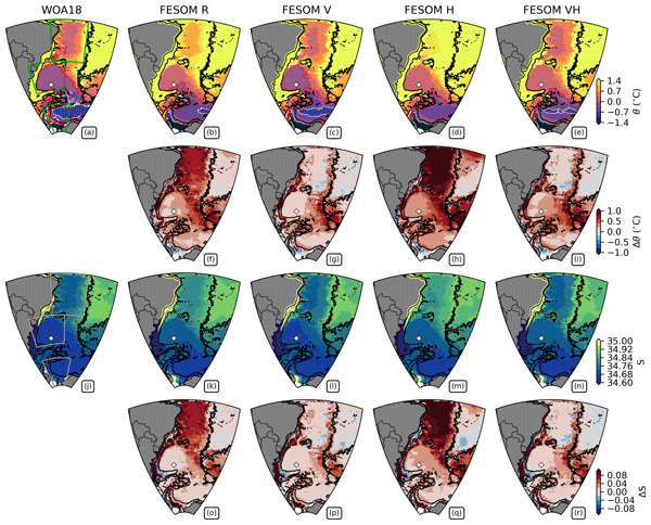
Line 377: remove 'a pattern common to all four FESOM simulations'. Response: The sentence has been removed as suggested. The paragraph was also revised to improve the description of the temperature distribution and the comparison with the previously evaluated models. (Line 457)
Lines 385-389: This paragraph is somewhat difficult to follow and would benefit from clarification. If its purpose is to compare the first four models with FESOM R to link the results from the FESOM simulations to the different performance between the models due to the different resolution – if it is what the authors are trying to demonstrate, I would suggest moving it to the discussion. If so, a similar figure could be made but this time of the difference of the four models with the different FESOM simulations (only for temperature). Response: We appreciate the reviewer's suggestion. The purpose of this paragraph is not to attribute the differences among ECCO, SODA, GLORYS, and OFES, nor to establish a direct one-to-one correspondence between these products and the FESOM experiments. Instead, the reference simulation (FESOM R) is first compared with the previously evaluated products to demonstrate that it reproduces the main recurring limitations identified in the intercomparison, thereby providing an appropriate baseline for the controlled resolution experiments. We therefore chose to retain this comparison within the Results section, as it establishes the logical transition between the intercomparison and the subsequent sensitivity experiments. The text has been revised to better clarify this objective and to emphasize that the controlled FESOM experiments are intended to investigate the role of grid resolution in the recurring limitations identified across the products, rather than to explain the differences among the products themselves. (Line 462-475)
Line 393: please remove 'comparable pattern obtained with GLORYS (Fig. 2d)'. Response: The sentence has been removed as suggested. (Line 479-480)
Line 397: please remove 'resembling the pattern observed in SODA (Fig. 2c), but with higher temperatures'. Response: The sentence has been removed as suggested.(Line 485)
Lines 405-410: move the paragraph after the salinity sigma4 descriptions and if possible add some references to support your reasoning. Response: We thank the reviewer for this suggestion. We agree that this paragraph is better placed after the discussion of the salinity and density fields, as it synthesizes the overall pattern of the four FESOM experiments rather than describing an individual simulation. Accordingly, we moved the paragraph to the end of the subsection, where it now serves as a synthesis of the results and their interpretation. We also revised the text to better emphasize the physical mechanism suggested by the experiments, namely that increased vertical resolution improves the representation of abyssal overflow pathways across the major bathymetric sills connecting the Weddell Sea, Argentine Basin, and Brazil Basin. Regarding the interaction between horizontal resolution and the Gent–McWilliams parameterization, we now present this as a possible explanation rather than a demonstrated mechanism, as this aspect was not directly investigated in the present study. (Line 517-538)
Figure 8 – caption: please include the description of the colorbars in the caption. As mentioned previously the authors might consider replacing the first colorbar to depth instead number of points. Response: The figure caption has been revised to include a description of both colorbars. We have retained the original color scale based on the number of points, as explained in our response to the previous comment.
Line 486: please include the value of the correlation. 0.8 is very high, any idea why FESOM R is reproducing the pattern so well for CLIVAR? Response: We have included the correlation value (r = 0.75) in the revised manuscript. Although this is a very high correlation, we do not have sufficient evidence to attribute it to a specific characteristic of the FESOM R configuration. Reproducing the phase of the observed temporal variability at a single mooring is a particularly demanding test for a global ocean model, especially within a narrow abyssal channel. While the configurations with enhanced vertical resolution (FESOM V and FESOM VH) provide a more realistic representation of the mean abyssal state and the magnitude of the observed variability across all mooring sites and periods, the correlations vary substantially among the individual mooring records. For example, FESOM R shows the highest correlation during the CLIVAR period but almost no correlation during the E2 period, whereas FESOM V exhibits the opposite pattern. Similar site-to-site variability is also found among the other evaluated products. We therefore added a paragraph to the manuscript clarifying that correlation at an individual mooring should not be interpreted as evidence of superior overall model performance.(Line 630-634)
Line 492: add correlation value. Response: We revised the section comparing the model results with the mooring observations. All correlation values are now explicitly reported in the text.
Line 493: where are the RMSE values? Response: We have revised the captions of Figs. 5 and A3 to clarify that the gray arcs represent the normalized RMSE.
Line 499: the highest correlation value is about 0.2 I think which does not show any correlation. The author might want to change the sentence to highlight the fact that the four simulations do not show any correlation with observations. Response: We agree and have revised the text accordingly. Rather than emphasizing the highest correlation coefficient among the simulations, we now state that none of the four simulations reproduced the observed temporal variability with significant skill. (Line 630-634)
Supplements: the name of the figures do not match the ones in the main text. Response: The references to the figures in the appendix have been revised. Now only one appendix exists and it contains all figures.
Data availability: Copernicus and OFES2 links do not get to the right pages. Also none of the zenodo links worked. Response: We revised Copernicus and OFES2 links. Zenodo token links are now available.
Video supplement: I wasn't able to access the video. Response: Thank you for pointing this out. We verified that the video supplement is available on the journal website. It may have been temporarily inaccessible during the review process.
Suggestions
Table 1: maybe the CTD data could also be added in Table 1. Response: We thank the reviewer for the suggestion. However, we chose to retain Table 1 as a summary of the mooring datasets only because the CTD observations represent a fundamentally different type of measurement. Including both datasets in a single table would therefore require several non-applicable fields and reduce the clarity of the presentation. Instead, both observational datasets are described together in Section 2.1, where their different characteristics and roles in this study are explained.
Figure 1: I would have found it helpful if the figure was also including a map of the bathymetry with the location of the Vema Channel and a rough schematic of the circulation. Response: We have revised Figure 1 to explicitly identify the Vema Channel, and add a schematic of the main abyssal circulation pathways.
Sections 2.3-2.5: To avoid the repletion about the atmospheric forcing, the 3 models could be under the same subsection 'Reanalysis models'. Response: We agree that the atmospheric forcing is repeated in the descriptions of the three reanalysis products. However, we prefer to retain the current organization because each subsection provides a complete description of the corresponding model, allowing readers to find all relevant information for a given product in a single place. We believe this structure improves readability and makes it easier to locate the characteristics of each model.
Table 3: the authors could consider adding the mooring mean and trend in the table. Response: We thank the reviewer for this suggestion. Table 3 was designed to summarize the comparison with the CTD observations, including the long-term temperature trends. As our trend analysis focuses on long-term changes, we did not include trends from the mooring records, which cover much shorter periods. Instead, the mooring analysis emphasizes mean temperature, variability, and correlation.
Section 3: A table summarising what each model is able or not to represent would be very valuable. Response: We appreciate the suggestion. Rather than adding a summary table, we revised the manuscript to better integrate the intercomparison with the subsequent FESOM experiments. The recurring characteristics identified across the evaluated products are now directly used to motivate the controlled experiments, which investigate whether these common patterns can be reproduced and explained through systematic changes in grid resolution.
Section 4: A table summarising the results would also be great! Response: We updated the Conclusions (Now Summary and conclusions) to provide a concise synthesis of the main findings of the four FESOM experiments, serving the same purpose as the proposed summary table.
-
AC1: 'Reply on RC1', Daniel Santos, 18 Aug 2026
-
RC2: 'Comment on egusphere-2026-2319', Anonymous Referee #2, 14 Jul 2026
The comment was uploaded in the form of a supplement: https://egusphere.copernicus.org/preprints/2026/egusphere-2026-2319/egusphere-2026-2319-RC2-supplement.pdf
-
AC2: 'Reply on RC2', Daniel Santos, 18 Aug 2026
We sincerely thank the reviewers for their careful evaluation of our manuscript and for their constructive comments and suggestions. We have carefully considered all remarks and substantially revised the manuscript accordingly.
The most significant revision was to strengthen the connection between the intercomparison of the evaluated ocean models and the controlled FESOM experiments. The revised manuscript now establishes clearly that the intercomparison is intended to identify recurring and model-specific limitations in the representation of abyssal waters, whereas the FESOM experiments provide a controlled framework to investigate whether changes in horizontal and vertical grid resolution can explain these recurring deficiencies. To reinforce this connection, the role of the reference configuration (FESOM R) is now explicitly introduced as a baseline that reproduces the main limitations identified in the intercomparison before assessing the effects of the controlled resolution changes. A detailed point-by-point response to all comments is provided below. All modifications to the manuscript have been highlighted using track changes.
The manuscript by Santos et al. investigates the influence of horizontal and vertical grid resolution on the representation of abyssal waters by evaluating three ocean reanalyses (ECCO, SODA, and GLORYS) and one forward ocean model (OFES2) from the Southern Ocean to the Brazilian Basin. The manuscript is well organized and clearly written. I recommend its acceptance for publication after moderate revisions.
Major Comments:
1. The WOA is a robust climatology representing the long-term mean state of the global ocean. However, it is generated using optimal interpolation, meaning that the observational coverage is spatially irregular. Since WOA18 is used as the primary reference for model evaluation, the authors should consider showing the distribution of observations (or data coverage) within the study area, as well as the estimated error field. For example, in Figure 2a, to what extent is the cold tongue surrounding the Antarctic continental shelf supported by observations, and how much is simply an artifact of the interpolation procedure? This information is important for assessing the reliability of the comparisons presented throughout the manuscript. Response: We thank the reviewer for this suggestion. We have added a new figure to the Appendix (Fig. A1) showing the spatial distribution of hydrographic profiles used to construct WOA18 within our study region. In addition, we have revised Section 2.2 to explicitly refer readers to this figure. We have also corrected our interpretation of the warm band along the Antarctic continental slope, which was incorrectly attributed to the spatial resolution of WOA18 in the previous version of the manuscript. The revised text recognizes this feature as consistent with the natural hydrographic structure of the Weddell Sea, where Warm Deep Water occupies the continental slope.
2. The description of the numerical models should be expanded to include additional information on bathymetry and lateral boundary conditions. Furthermore, I encourage the authors to discuss the fundamental differences between forward ocean models and ocean reanalyses, which would help the readers better understand the expected differences in variability and long-term trends, and, more importantly, the aspects that should be considered when comparing reanalyses with forward ocean models. Finally, some discussion of how differences in model configuration (e.g., atmospheric forcing, vertical and horizontal mixing parametrizations, sea-ice representation, among others) may contribute to the differences found in this study would strengthen the scientific impact of the manuscript. Response: Following the recommendation, we expanded the description of the numerical models by including additional information on model bathymetry, atmospheric forcing, sea-ice representation, and other relevant aspects of the model configuration when available in the primary model references. We also added a short methodological discussion highlighting the fundamental differences between ocean reanalyses and forward simulations and the considerations required when comparing these products. Finally, we revised the introduction to the controlled FESOM experiments to explicitly acknowledge that the evaluated products differ in several aspects beyond grid resolution, and to clarify that the intercomparison alone cannot isolate the contribution of individual model components. This motivation is now used to introduce the controlled FESOM experiments, in which only grid resolution is modified while all other model components remain unchanged.
Minor Comments:
1. Line 30: Should this reference be Santos et al. (2026)? In addition, is this really the first published study reporting this result? Response: We have corrected the citation to Santos et al. (2026). We also agree that the original observation should not be attributed solely to this study. Therefore, we now cite both Coles et al. (1996), which first documented this result, and Santos et al. (2026), which revisits and updates those findings using recent observations.(Line 33-44)
2. Lines 53-64: A recent study by Noro et al. (2025), Variability of the Weddell Sea Deep Waters in the GLORYS12v1 Reanalysis, should be included in this background discussion. Response: following the reviewer's suggestion, we have incorporated Noro et al. (2025) into the Introduction. (Line 67-69).
3. Fig.1: It would be helpful to include latitude labels on the y-axis. Response: We added the coordinates.
4. Table 2: It would be useful to include the temporal resolution of each model. Response: Rather than adding the temporal resolution to Table 2, we have included this information in the corresponding descriptions of each model in the text. All analyses in this study were performed using monthly model outputs.
5. Lines 188-191: Since the authors acknowledge the limited spatial resolution of WOA18, it is not entirely clear how the comparisons should be interpreted. For example, WOA18 shows temperatures near -0.7°C in the central Weddell Sea, whereas OFES2 simulates colder waters. Given that WOA18 has a horizontal resolution of 0.25° while OFES2 has a resolution of 0.1°, can WOA18 confidently be considered the reference in this region? Response: As discussed in our response to Major Comment 1, we have added a new figure to the Appendix (Fig. A1) showing the spatial distribution of hydrographic profiles used to construct WOA18 and revised Section 2.2 accordingly. We also corrected our previous interpretation of the warm band along the Antarctic continental slope, which had been incorrectly attributed to the spatial resolution of WOA18. The revised text recognizes this feature as consistent with the natural hydrographic structure of the Weddell Sea, where Warm Deep Water occupies the continental slope.
With regard to the use of WOA18 as a reference, we acknowledge that its representation of the abyssal Weddell Sea should be interpreted in the context of the available hydrographic observations. Nevertheless, WOA18 remains the most comprehensive observational climatology currently available for basin-scale comparisons in this region.
Both WOA18 and the repeated hydrographic observations along the A12 section (Dotto et al., 2014; Fig. 4) consistently indicate the absence of the widespread abyssal temperatures below −1 °C simulated by OFES. We recognize, however, that this is not an independent validation, since WOA18 is constructed from the available hydrographic observations, including those from the A12 section. Taken together, the consistency between the climatology and the repeated hydrographic measurements supports the use of WOA18 as an appropriate observational reference for evaluating the basin-scale abyssal hydrography in this region and reinforces our conclusion that OFES produces an unrealistically cold representation of the abyssal Weddell Sea.
6. Figure 2.: I suggest changing the continent color to dark gray, as the Antarctic continent is difficult to distinguish from the light-red color scale. In addition, consider outlining the Argentine and Brazilian basins with rectangles (at least in the WOA18 panels) to facilitate interpretation. Response: We have changed the continent color to dark gray to improve the contrast with the temperature bias color scale. We have also added rectangles to the WOA18 panels to delineate the Brazil Basin, Argentine Basin, and Weddell Sea, and updated the figure caption accordingly.
7. Why were HYCOM products not included instead of ECCO or SODA? Recent HYCOM analyses have shown improved performance in representing abyssal circulation and water masses. Response: The selected products were intended to provide a representative sample of widely used ocean products rather than an exhaustive collection of available reanalyses and models. By combining products with different model formulations and data assimilation approaches, we sought to identify recurring limitations that are not specific to a single product. The recurring limitations identified across these products motivated the subsequent FESOM 2 experiments, which were designed to isolate the influence of horizontal and vertical grid resolution. Including HYCOM would provide an interesting additional comparison and broaden the intercomparison, but we do not expect it to affect the main conclusions regarding the recurring limitations identified across the selected products and the role of model resolution.
8. Fig.5: I suggest changing the color used for either ECCO or OFES, since the two shades of green are difficult to distinguish. Also, am I the only one who cannot identify the GLORYS triangles in the Taylor diagrams? Response: We have revised the color scheme of Fig. 5 to improve the distinction among the different products. GLORYS consistently exhibits the largest standard deviation, placing its markers farther from the reference point than those of the other products. Increasing the size of the Taylor diagrams sufficiently to clearly distinguish these markers would have compromised the layout and readability of the complete figure. Therefore, the full extent Taylor diagrams are also presented in Appendix Fig. A3, where all markers can be identified.
9. Although FESOM-VH provides the best representation of abyssal water properties and inter-basin connectivity, its correlation coefficient with the moored observations is among the lowest. Do the authors have an explanation for why FESOM-VH reproduces the observed temporal variability so poorly despite its otherwise good performance? Response: Although the configurations with enhanced vertical resolution (FESOM V and FESOM VH) provide a more realistic representation of the mean abyssal state and the magnitude of the observed variability over all mooring sites and periods, we do not have sufficient evidence to attribute the comparatively low correlation of FESOM VH at individual mooring locations to a specific process. Reproducing the phase of the observed temporal variability at a single mooring is a particularly demanding test for a global ocean model, especially within a narrow abyssal channel, and the correlations vary substantially among the different mooring records. For example, FESOM R shows the highest correlation during the CLIVAR period but almost no correlation during the E2 period, whereas FESOM V exhibits the opposite pattern. Similar site-to-site variability is also found among the other evaluated products. We therefore added a paragraph to the manuscript clarifying that correlation at an individual mooring should not be interpreted as evidence of superior overall model performance. (Line 630-634)
10. Line 499: A correlation coefficient of approximately 0.2 should not be considered statistically meaningful. Therefore, I suggest rephrasing the sentence rather than emphasizing that this was "the highest value." Instead, it would be more appropriate to highlight that none of the four simulations reproduced the temporal variability observed by the moorings with significant skill. Response: We agree and have revised the text accordingly. Rather than emphasizing the highest correlation coefficient among the simulations, we now state that none of the four simulations reproduced the observed temporal variability with significant skill. (Line 630-634)
11. Although the study provides a comprehensive analysis of eight simulations, the rationale for selecting each OGCM is not clearly explained, nor is the “motivation” (see line 521) to perform four targeted experiments with FESOM 2. It would be interesting to have this discussed in the manuscript. Moreover, the analyses were well conducted throughout the study area; however, I cannot see a clear focus on the Vema Channel, it appears to be just another analysis site. In practice, the manuscript focuses on the representation of abyssal water masses in numerical models. Therefore, I suggest removing "A Focus on Vema Channel" from the title. Response: We revised the manuscript to clarify both the rationale for the selected ocean products and the motivation for the FESOM 2 experiments. Specifically, we now state that ECCO, SODA, GLORYS, and OFES were selected as widely used ocean products representing different model formulations, including ocean reanalyses with distinct data assimilation approaches and a forward ocean model. We also revised the Introduction to explicitly explain that the recurring limitations identified across these products motivate the targeted FESOM 2 experiments, which are designed to isolate the respective influences of horizontal and vertical grid resolution on the representation of abyssal water properties and inter-basin connectivity.
We also agree that the previous title overemphasized the Vema Channel relative to the overall scope of the study. To better reflect the main objective of the manuscript, we removed the phrase "A Focus on Vema Channel" from the title. (Line 76-89)
12. There appears to be some inconsistency in the naming of the additional figures, with references alternating between "Appendix" and "Supplementary Material." Please check and standardize the terminology. Response: Now the manuscript refers correctly to video supplementary material and to the figures in appendix A.
13. Although the manuscript focuses on the impact of model resolution, I felt that it lacks a more direct conclusion regarding which reanalysis provides the best representation of abyssal waters and which numerical model performs best overall. A concise synthesis of the relative strengths and weaknesses of each product would help readers better appreciate the main findings and practical implications of the study. Response: We appreciate the reviewer's suggestion. We agree that a ranking of the evaluated products could be useful for some applications. However, the primary objective of this study is not to identify a best-performing model, but rather to investigate the recurring limitations shared across independent ocean products and to examine, through controlled FESOM experiments, whether these limitations can be explained by grid resolution. We recognize that this distinction was not sufficiently clear in the previous version of the manuscript. Therefore, we revised the text throughout the Results, Discussion, and Conclusions to more clearly establish the role of the intercomparison as the motivation for the controlled FESOM experiments. Because model performance depends on the specific diagnostic considered, we chose to emphasize the recurring and model-specific biases identified in the intercomparison rather than establish an overall ranking of the evaluated products.
Citation: https://doi.org/10.5194/egusphere-2026-2319-AC2
-
AC2: 'Reply on RC2', Daniel Santos, 18 Aug 2026
Peer review completion


Interactive discussion
Status: closed
-
RC1: 'Comment on egusphere-2026-2319', Anonymous Referee #1, 10 Jun 2026
The comment was uploaded in the form of a supplement: https://egusphere.copernicus.org/preprints/2026/egusphere-2026-2319/egusphere-2026-2319-RC1-supplement.pdf
-
AC1: 'Reply on RC1', Daniel Santos, 18 Aug 2026
We sincerely thank the reviewers for their careful evaluation of our manuscript and for their constructive comments and suggestions. We have carefully considered all remarks and substantially revised the manuscript accordingly.
The most significant revision was to strengthen the connection between the intercomparison of the evaluated ocean models and the controlled FESOM experiments. The revised manuscript now establishes clearly that the intercomparison is intended to identify recurring and model-specific limitations in the representation of abyssal waters, whereas the FESOM experiments provide a controlled framework to investigate whether changes in horizontal and vertical grid resolution can explain these recurring deficiencies. To reinforce this connection, the role of the reference configuration (FESOM R) is now explicitly introduced as a baseline that reproduces the main limitations identified in the intercomparison before assessing the effects of the controlled resolution changes. A detailed point-by-point response to all comments is provided below. All modifications to the manuscript have been highlighted using track changes.
The study investigates the representation of abyssal waters in three reanalysis models (ECCO, SODA, and GLORYS) and one OGCM (OFES) across the region extending from the Weddell Sea—where deep and bottom waters are formed—to the Brazil Basin, where they flow northward. Model performance is evaluated against the WOA18 climatology as well as in situ observations (moorings and CTD data). This comprehensive assessment of existing reanalyses and models provides valuable insights for future studies in this region.
Given that the four models differ in their grid resolution, the authors further explore the impact of increased horizontal and bottom vertical resolution using additional simulations with FESOM. These experiments offer important insights into how model resolution affects the representation of deep and bottom waters, and more broadly, improve our understanding of the role of resolution in simulating ocean circulation and water mass properties.
The manuscript is well written, and the results clearly stated however the manuscript would benefit from a more extensive and defined discussion section.
Main/general comments
1. The model descriptions in the Methods section are quite brief, and some key information is currently missing. To help readers better understand the differences between the models, it would be beneficial to provide additional details beyond the grid configuration. In particular, the authors should consider including information on bathymetry, mixing parameterisations, boundary conditions, and any other relevant model components. This would make it easier to interpret the results and identify the sources of inter-model differences. Response: Following the recommendation, we expanded the description of the numerical models and other relevant aspects of the models configurations when available in the primary model references. (Sections 2.3-2.7)
2. The results presented are very interesting; however, their overall impact would be strengthened by a more in-depth discussion of the mechanisms driving the differences between the four models. While the FESOM simulations are used to explore the impact of horizontal and vertical resolution, the connection with the other models is not fully developed. Expanding this discussion would help readers understand how the FESOM-based findings relate to and explain the variability seen across the models.
It would also be useful to include a more explicit comparison of the five models in terms of their configurations, such as core model structure, bathymetry, data assimilation (including whether assimilation is performed in this region and which datasets are used), diffusivity and mixing schemes, dissipation, and sea-ice representation. These factors are likely to influence the simulation of deep waters and could provide valuable insight into the differences observed.
Additionally, a short paragraph discussing the limitations of the climatology and observational datasets used for validation—particularly in this region—would improve the robustness of the study.
Finally, incorporating references on the impact of model resolution on ocean circulation could further support and contextualise the interpretation of the results. Response: We thank the reviewer for this important comment. We have substantially revised the manuscript to strengthen the connection between the intercomparison and the controlled FESOM experiments. Rather than attributing differences among ECCO, SODA, GLORYS, and OFES to individual model components, we now use FESOM R as a baseline to assess whether the recurring limitations identified across the evaluated simulations can also arise in an independent model. The subsequent experiments isolate the influence of horizontal and vertical grid resolution while keeping the other model components unchanged. We also expanded the discussion of the mechanisms underlying the results, particularly the role of abyssal thermal structure and overflow pathways through major bathymetric sills.
We further expanded the description of the numerical models by including additional information on model formulation, bathymetry, atmospheric forcing, sea-ice representation, mixing schemes, and data assimilation, when available in the primary model references. We also added more contextualization of the limitations found during the intercomparison of the models.
To better document the validation datasets, we included a new figure showing the spatial distribution of the hydrographic observations used in WOA18.
Additional references discussing the influence of model resolution on abyssal circulation and overflow representation have also been incorporated into the manuscript.
3. In general, the figure captions are missing information. Please make sure that all the features on the figure are described in the caption to help the reader navigate the figure. Response: We have revised all figure captions to ensure that the features shown in each figure are fully described
Comments
Line 42: it is not clear if the 3 latitudes are the latitudes of the moorings. Please rephrase. Response: The text has been revised to improve comprehension. (Line 45-47)
Line 81: can the authors provide more information regarding the frequency of the measurements, if they are all done on the same month, etc. Response: Additional information regarding the CTD sampling strategy has been added. (Line 100-101)
Lines 83-84: the mention of the PIES instruments at the same location is a bit confusing as those observations are not used in this study. Please rephrase or edit the sentence. Response: The text has been rephrased as suggested. (Line 102)
Figure 1: It would be helpful to have latitude and longitude on the maps. Response: We added the coordinates.
Figure 1 caption: 'Green diamonds mark CTD sites' – add CTD. Response: The figure caption has been revised as suggested.
Table 1: for SAMBAR, is it a typo the year '2020' in the last column?. Response: Yes, this was a mistake. The year has been corrected in the revised manuscript. We also corrected the CLIVAR sampling dates in Table 1.
Line 104: are the outputs snapshots or averages? The authors could mention that only (I suppose) monthly outputs have been used in this study. Response: The manuscript has been revised to clarify that only the monthly ECCO outputs were used in the present study. (Line 125-126)
Lines 106-107: It is unclear if this sentence 'The product …' refers to the atmospheric forcing or to the model. Response: The text was revised to clarify that the sentence refers to the SODA product rather than to the atmospheric forcing. The relevant information was reorganized within the paragraph to improve readability and avoid ambiguity. (Line 136-143)
Line 126: The format of the reference is wrong. First names are displayed instead of the last name of the authors. Response: The issue was caused by an incorrectly formatted BibTeX entry, in which the authors' first and last names were reversed. The reference has been corrected, and the citation now displays the authors' surnames properly.
Line 131: 'We assess…' it feels like the sentence is incomplete. Response: The sentence has been revised to improve clarity and completeness. (Line 160)
Section 2.6: can the authors add more details about the initial conditions and forcing of the ocean? Response: Additional information regarding the model initial conditions and atmospheric forcing has been added. The manuscript now specifies the source of the initial temperature and salinity fields and clarifies that the simulation is forced by the JRA55-do atmospheric dataset.
Line 135: is '1958-2019' the period of the atmospheric data or of the model? Please clarify and rephrase. Response: The text has been revised to clarify that the period 1958--2016 refers to the OFES simulation rather than to the atmospheric forcing dataset. (Line 167)
Line 135: what do the authors mean by 'the model focuses on the upper ocean'? The reader might wonder why this model would be used in this study if it is not made for deep ocean. The last 3 sentences would benefit some rewriting to improve the message. Response: As pointed out, this statement could lead to a misunderstanding of the model capabilities. Our intention was to highlight that the vertical resolution is enhanced near the surface. To avoid ambiguity, we removed this statement and rewrote the final sentences to provide a more descriptive description of the vertical grid configuration. (Section 2.6)
Line 155: please replace 'first' by 'reference' and delete '(from reference)'. Response: The suggested change was adopted and the corresponding descriptions of the other simulations were revised accordingly to ensure consistency throughout the manuscript. (Section 2.7)
Line 158: It might be better to have the depth in meters to be coherent with the other models. Response: The vertical coordinate was incorrectly reported in dbar. This has been corrected to meters throughout the manuscript for consistency with the FESOM vertical coordinate system and with the descriptions of the other models.
Line 159: Can the authors explain what they mean by 'the base horizontal resolution was set to 30 km'?. Response: The text has been revised to clarify that 30 km corresponds to the nominal horizontal resolution over most of the global domain, while the mesh is refined in selected regions and toward higher latitudes. (Line 196-198)
Line 161/167: replace 'from' by 'for'. Response: As described in the response to a previous comment (Line 155), the nomenclature of the FESOM experiments was revised throughout the manuscript. Consequently, the parenthetical expressions were removed and the corresponding passages were reformulated for clarity and consistency.
Line 163: is this simulation less deep than the other one? How many more levels are added? Response: Yes, FESOM V is shallower than FESOM R by 2000 m (5350 vs. 7350 m). However, it adds 20 more vertical levels (105 → 125), all concentrated between 3800 and 5350 m, yielding ~50 m resolution near the seafloor in that range. For reference, FESOM R has only 13 levels spread across the much larger 3800–7350 m range. To make this trade-off more explicit, we also revised Table 2 by: (i) adding a "Max depth (m)" column so the difference in vertical extent between simulations is immediately visible, (ii) renaming the "Layers (3800–6000)" column to "Levels (3800 m – max depth)", and (iii) adding a "Vert. spacing below 3800 m" column, which shows that the reanalyses have spacings of ~210–440 m in this depth range, further contextualizing the ~50 m resolution achieved by FESOM V. We also corrected the unit from dbar to m throughout, as the FESOM vertical coordinate is in meters. (Line 201-204)
Table 2: add 'atmospheric' with 'forcing'. Also, only for the table, the authors might choose to have all resolutions in km or in degrees for coherence between the models. Response: We added 'atmospheric' before 'forcing' in the Table 2 header. Regarding resolution units, we kept the native units of each model and added a footnote with km equivalences for SODA, GLORYS, and OFES to facilitate comparison.
Lines 189-191: 'This feature…' It would be interesting to expend this in the discussion on the limitations of the climatology for validating the models. Response: We have added a new figure to the Appendix (Fig. A1) showing the spatial distribution of hydrographic profiles used to construct WOA18 within our study region. In addition, we have revised Section 2.2 to explicitly refer readers to this figure, which provides context for the observational support underlying the objectively interpolated climatological fields used throughout this study. We have also corrected our interpretation of the warm band along the Antarctic continental slope, which was incorrectly attributed to the spatial resolution of WOA18 in the previous version of the manuscript. The revised text recognizes this feature as consistent with the natural hydrographic structure of the Weddell Sea, where Warm Deep Water occupies the continental slope.
Figure 2- caption: Can you clarify what the authors mean by 'total'? Response: We thank the reviewer for pointing this out. The term 'total' was unnecessary and has been removed from the caption.
Lines 246-261: This paragraph could be used later on to discuss the differences between models as it doesn't really compare with observations as the rest of the section. Response: We have clarified the objectives of Section 3.1 by revising its introductory paragraph. The revised text now explicitly states that the section compares the simulated abyssal water masses with in situ observations and the WOA18 climatology, and also examines the temporal evolution of the simulated density fields. This clarification better explains the scope of the section and the purpose of the temporal analysis. (Line 219-223)
Line 251/261: what do the authors means by 'the outputs are not continuous in time'? Is it not monthly outputs? If it is not, how is it taken in consideration in the different analyses?. Response: The statement has been clarified. All analyses were performed using monthly model outputs. The previous wording was misleading and has been revised to avoid suggesting that the temporal sampling of the simulations was discontinuous. (Line 294)
Lines 254-261: it would be interesting to understand these trends and their possible impact on the results. Response: Our interpretation is that the contrasting long-term trends reflect differences in the representation of abyssal connectivity between the Weddell, Argentine, and Brazil basins. When the propagation of abyssal waters through the interconnected deep basins is not adequately represented, the temporal evolution of abyssal properties becomes inconsistent between the source region and downstream basins. This interpretation is consistent with the controlled FESOM experiments, which show that improving the representation of abyssal pathways through increased vertical resolution substantially improves inter-basin connectivity.
Section 3.2: are the T-S diagrams an average of the points in the white boxes per level (from surface to bottom) or all grid points are represented? Also Fig. 3a and 3b are not directly described in the text, especially how it transitions from one to another. Response: We have added two clarifying passages to Section 3.2. The first clarifies that all grid points from the surface to 6000 m within the Argentine and Brazil basins are represented in the 2D histogram (not averages per level), and describes the interpolation procedure. The second describes the WOA18 reference panels (Figs. 3a and 3b) and explains the inter-basin transition. (Line 318-320) and (Line 321-326)
Line 272: if possible, please add the location of the Scottia Ridge on a map. Response: We have revised Figure 1 to include a schematic of the main abyssal circulation pathways. We did not explicitly label the South Scotia Ridge, as this would make the figure crowded. However, additional geographic features have been identified in the revised figure, making the location of the South Scotia Ridge easier to infer, as it forms the southern boundary of the Scotia Basin. In addition, we expanded the description of the overflow pathways in the Introduction to provide a clearer explanation of the propagation of Antarctic Bottom Water from the Weddell Sea until the western South Atlantic.
Figure 3: the authors might consider to change the colorbar to depth instead of number of points to highlight the location of the difference water masses on the vertical. Response: While coloring by depth would certainly provide valuable information, here we focus on a more fundamental assessment: whether the simulations correctly reproduce the observed distribution of water mass classes. The difference panels directly show whether a given simulation over- or underproduces certain θ–S classes relative to WOA18. For example, ECCO and SODA clearly fail to reproduce the densest water classes in both basins. For models with a more realistic vertical structure, such as GLORYS and OFES, a depth-colored representation could add further understanding. Nevertheless, even within the current framework, inferences about the vertical distribution are possible: for instance, the higher point counts at the densest portion of the diagram in OFES (Fig. 3q) suggest that its deepest layers are occupied by colder and denser waters, consistent with what a depth-colored diagram would show. We therefore retain the volumetric representation as it allows a direct inter-model comparison of water mass property biases.
Figure 3 – caption: the colorbars are not explained in the caption. Response: The colorbar descriptions have been added to the caption.
Line 289: the use of the word 'discontinuity' here is not clear to me. Can the authors clarify what they mean by this. Response: We have clarified the meaning of discontinuity in the text by explicitly stating that it refers to the abrupt change in abyssal water properties between the Argentine and Brazil basins. (Line 341)
Line 295: again, I am confused with the use of 'discontinuities'. Are they expected to be the same?. Response: We have revised the text to avoid the ambiguous term discontinuities. The opening of this subsection now directly introduces the objective of examining where and how the changes in abyssal water properties develop along the northward pathway. (Line 346)
Section 3.3: at which latitude is the cross-section? Have the authors considered the neared grid point for each model or did they interpolated the results to the exact same latitude? Response: The section for each model corresponds to the nearest available latitude to 31.3°S in that model's native grid. Since each model has a different horizontal resolution, the actual latitude of the extracted section differs slightly between products. No interpolation was applied to enforce a common latitude. We have revised the text and figure caption to clarify this point. (Line 350-352)
Line 305: Is the absence of the Vema Channel only at this latitude or is it not at all present? Having looked at a map, the Vema Channel extendens from 28S to 32S. Response: Thank you for pointing this out. After revisiting the horizontal temperature distribution at the model levels closest to the maximum depth of the Vema Channel (Attached figure), we realized that our original interpretation was incorrect. The Vema Channel is present in all models, but it is poorly represented, with substantial differences in the depth of the deepest model levels occupying the channel. We have therefore revised the manuscript to replace "absent" with "poorly represented" and Figure 4 was updated to show this more explicitly. (Line 360)
Figure caption: Potential temperature (θ) at two abyssal levels and their difference (Δθ = θ_upper − θ_lower, °C) for January 1993 over the study area. (a, d, g, j) and (b, e, h, k) show θ at the shallower and deeper levels, respectively. (c, f, i, l) show Δθ between the two levels. Depth pairs are approximately 4264–4640 m (ECCO), 4556–4765 m (SODA), 4405–4833 m (GLORYS), and 4389–4671 m (OFES).
Line 317: could it also be due to a bathymetry blockage? Response: Yes, this pattern is also consistent with a bathymetric blockage. As shown in the figure above, the coldest abyssal waters in ECCO are largely confined south of the Vema Channel and do not propagate into the Brazil Basin. To further investigate this hypothesis, we added the new Appendix Fig. A4, which shows the mean vertical temperature structure in the Argentine Basin. The figure reveals that, although ECCO is the coldest model at the deepest level, it exhibits a relatively strong vertical temperature gradient in the abyss. Consequently, at the depth of the Vema Channel sill, substantially warmer waters are available for northward export into the Brazil Basin, while the coldest bottom waters remain confined below the sill. This interpretation is also supported by the mooring comparison (Fig. 6), where Site D, located in the deeper part of the channel and compared with the 4640 m model level, exhibits substantially colder temperatures than Site C, located in a shallower region and compared with the 4264 m model level. We have revised the manuscript accordingly. (Line 371-376)
Lines 318-319: Any ideas why OFES presents a cooling in the Vema Channel and the Brazil Basin? Response: To investigate this pattern, we added a new figure to the appendix (Fig. A4), which shows the mean vertical temperature profiles in the Argentine Basin. The additional analysis reveals that, although OFES is relatively warm at its deepest model level, it exhibits a weaker abyssal vertical temperature gradient than the other products. Consequently, at the depth corresponding to the Vema Channel sill, OFES exports colder waters from the Argentine Basin into the Brazil Basin than the other simulations. This provides a consistent explanation for the cooling simulated in both the Vema Channel and the Brazil Basin. (Line 371-376)
Figure 4 – caption: please move (a), (b), etc before the model name. On a different note, is there a particular reason for why the authors have highlighted the isotherm 0.04? Response: We have revised the caption by placing the panel labels ((a), (b), etc.) before the corresponding model names. The 0.04°C isotherm was originally included to facilitate the comparison of the abyssal temperature structure between the FESOM V and FESOM VH experiments. However, we agree that it does not provide substantial additional information in the context of this figure. Therefore, we have removed this isotherm from the revised version.
Lines 325/347: please replace 'four products' by 'four models' for clarity. All ‘products’ have been replaced by ‘models’ in the text. Response: All occurrences of “products” have been replaced by “simulations” throughout the manuscript for consistency and clarity.
Line 327: It is very interesting that GLORYS shows such a high monthly variability especially in the deep ocean. Do the authors have any ideas why it is happening? It seems very strange. Could they be snapshots and the other models are monthly average? Response: We investigated this possibility and confirmed that the GLORYS product analyzed in this study provides monthly mean fields rather than instantaneous snapshots. Therefore, the enhanced variability cannot be attributed to differences in the temporal averaging of the archived outputs. Following the reviewer's broader suggestion, we also expanded the model descriptions in the Methods section to include additional information on model configurations. Nevertheless, because the evaluated products differ simultaneously in several aspects, it is not possible to attribute the enhanced variability to a single factor based on the present analysis. Identifying the origin of these intermittent fluctuations would require a dedicated model intercomparison study specifically designed to isolate the effects of these individual components.
Figure 5: On the Taylor diagrams the authors could consider plotting the normalised standard deviation instead of the standard deviation (normalised by the reference). On another note, what are the thick grey lines represent? If they are the standard deviation, why do the not align with the thin lines? Regarding the time series for SAMBA, how can you have SODA (finishing in 2019 in Table 1) and GLORYS (finishing in 2018)? Response: We have revised the Taylor diagrams to display the normalized standard deviation. We have also revised the captions of Figs. 5 and A5 to clarify that the gray arcs represent the normalized RMSE. In addition, we corrected the temporal coverage of the GLORYS and SODA datasets in the manuscript to match the periods used in this study.
Figure 5 – caption: 'temperature monthly time series' – add 'monthly'. Response: The text has been corrected as suggested.
Line 377: remove 'a pattern common to all four FESOM simulations'. Response: The sentence has been removed as suggested. The paragraph was also revised to improve the description of the temperature distribution and the comparison with the previously evaluated models. (Line 457)
Lines 385-389: This paragraph is somewhat difficult to follow and would benefit from clarification. If its purpose is to compare the first four models with FESOM R to link the results from the FESOM simulations to the different performance between the models due to the different resolution – if it is what the authors are trying to demonstrate, I would suggest moving it to the discussion. If so, a similar figure could be made but this time of the difference of the four models with the different FESOM simulations (only for temperature). Response: We appreciate the reviewer's suggestion. The purpose of this paragraph is not to attribute the differences among ECCO, SODA, GLORYS, and OFES, nor to establish a direct one-to-one correspondence between these products and the FESOM experiments. Instead, the reference simulation (FESOM R) is first compared with the previously evaluated products to demonstrate that it reproduces the main recurring limitations identified in the intercomparison, thereby providing an appropriate baseline for the controlled resolution experiments. We therefore chose to retain this comparison within the Results section, as it establishes the logical transition between the intercomparison and the subsequent sensitivity experiments. The text has been revised to better clarify this objective and to emphasize that the controlled FESOM experiments are intended to investigate the role of grid resolution in the recurring limitations identified across the products, rather than to explain the differences among the products themselves. (Line 462-475)
Line 393: please remove 'comparable pattern obtained with GLORYS (Fig. 2d)'. Response: The sentence has been removed as suggested. (Line 479-480)
Line 397: please remove 'resembling the pattern observed in SODA (Fig. 2c), but with higher temperatures'. Response: The sentence has been removed as suggested.(Line 485)
Lines 405-410: move the paragraph after the salinity sigma4 descriptions and if possible add some references to support your reasoning. Response: We thank the reviewer for this suggestion. We agree that this paragraph is better placed after the discussion of the salinity and density fields, as it synthesizes the overall pattern of the four FESOM experiments rather than describing an individual simulation. Accordingly, we moved the paragraph to the end of the subsection, where it now serves as a synthesis of the results and their interpretation. We also revised the text to better emphasize the physical mechanism suggested by the experiments, namely that increased vertical resolution improves the representation of abyssal overflow pathways across the major bathymetric sills connecting the Weddell Sea, Argentine Basin, and Brazil Basin. Regarding the interaction between horizontal resolution and the Gent–McWilliams parameterization, we now present this as a possible explanation rather than a demonstrated mechanism, as this aspect was not directly investigated in the present study. (Line 517-538)
Figure 8 – caption: please include the description of the colorbars in the caption. As mentioned previously the authors might consider replacing the first colorbar to depth instead number of points. Response: The figure caption has been revised to include a description of both colorbars. We have retained the original color scale based on the number of points, as explained in our response to the previous comment.
Line 486: please include the value of the correlation. 0.8 is very high, any idea why FESOM R is reproducing the pattern so well for CLIVAR? Response: We have included the correlation value (r = 0.75) in the revised manuscript. Although this is a very high correlation, we do not have sufficient evidence to attribute it to a specific characteristic of the FESOM R configuration. Reproducing the phase of the observed temporal variability at a single mooring is a particularly demanding test for a global ocean model, especially within a narrow abyssal channel. While the configurations with enhanced vertical resolution (FESOM V and FESOM VH) provide a more realistic representation of the mean abyssal state and the magnitude of the observed variability across all mooring sites and periods, the correlations vary substantially among the individual mooring records. For example, FESOM R shows the highest correlation during the CLIVAR period but almost no correlation during the E2 period, whereas FESOM V exhibits the opposite pattern. Similar site-to-site variability is also found among the other evaluated products. We therefore added a paragraph to the manuscript clarifying that correlation at an individual mooring should not be interpreted as evidence of superior overall model performance.(Line 630-634)
Line 492: add correlation value. Response: We revised the section comparing the model results with the mooring observations. All correlation values are now explicitly reported in the text.
Line 493: where are the RMSE values? Response: We have revised the captions of Figs. 5 and A3 to clarify that the gray arcs represent the normalized RMSE.
Line 499: the highest correlation value is about 0.2 I think which does not show any correlation. The author might want to change the sentence to highlight the fact that the four simulations do not show any correlation with observations. Response: We agree and have revised the text accordingly. Rather than emphasizing the highest correlation coefficient among the simulations, we now state that none of the four simulations reproduced the observed temporal variability with significant skill. (Line 630-634)
Supplements: the name of the figures do not match the ones in the main text. Response: The references to the figures in the appendix have been revised. Now only one appendix exists and it contains all figures.
Data availability: Copernicus and OFES2 links do not get to the right pages. Also none of the zenodo links worked. Response: We revised Copernicus and OFES2 links. Zenodo token links are now available.
Video supplement: I wasn't able to access the video. Response: Thank you for pointing this out. We verified that the video supplement is available on the journal website. It may have been temporarily inaccessible during the review process.
Suggestions
Table 1: maybe the CTD data could also be added in Table 1. Response: We thank the reviewer for the suggestion. However, we chose to retain Table 1 as a summary of the mooring datasets only because the CTD observations represent a fundamentally different type of measurement. Including both datasets in a single table would therefore require several non-applicable fields and reduce the clarity of the presentation. Instead, both observational datasets are described together in Section 2.1, where their different characteristics and roles in this study are explained.
Figure 1: I would have found it helpful if the figure was also including a map of the bathymetry with the location of the Vema Channel and a rough schematic of the circulation. Response: We have revised Figure 1 to explicitly identify the Vema Channel, and add a schematic of the main abyssal circulation pathways.
Sections 2.3-2.5: To avoid the repletion about the atmospheric forcing, the 3 models could be under the same subsection 'Reanalysis models'. Response: We agree that the atmospheric forcing is repeated in the descriptions of the three reanalysis products. However, we prefer to retain the current organization because each subsection provides a complete description of the corresponding model, allowing readers to find all relevant information for a given product in a single place. We believe this structure improves readability and makes it easier to locate the characteristics of each model.
Table 3: the authors could consider adding the mooring mean and trend in the table. Response: We thank the reviewer for this suggestion. Table 3 was designed to summarize the comparison with the CTD observations, including the long-term temperature trends. As our trend analysis focuses on long-term changes, we did not include trends from the mooring records, which cover much shorter periods. Instead, the mooring analysis emphasizes mean temperature, variability, and correlation.
Section 3: A table summarising what each model is able or not to represent would be very valuable. Response: We appreciate the suggestion. Rather than adding a summary table, we revised the manuscript to better integrate the intercomparison with the subsequent FESOM experiments. The recurring characteristics identified across the evaluated products are now directly used to motivate the controlled experiments, which investigate whether these common patterns can be reproduced and explained through systematic changes in grid resolution.
Section 4: A table summarising the results would also be great! Response: We updated the Conclusions (Now Summary and conclusions) to provide a concise synthesis of the main findings of the four FESOM experiments, serving the same purpose as the proposed summary table.
-
AC1: 'Reply on RC1', Daniel Santos, 18 Aug 2026
-
RC2: 'Comment on egusphere-2026-2319', Anonymous Referee #2, 14 Jul 2026
The comment was uploaded in the form of a supplement: https://egusphere.copernicus.org/preprints/2026/egusphere-2026-2319/egusphere-2026-2319-RC2-supplement.pdf
-
AC2: 'Reply on RC2', Daniel Santos, 18 Aug 2026
We sincerely thank the reviewers for their careful evaluation of our manuscript and for their constructive comments and suggestions. We have carefully considered all remarks and substantially revised the manuscript accordingly.
The most significant revision was to strengthen the connection between the intercomparison of the evaluated ocean models and the controlled FESOM experiments. The revised manuscript now establishes clearly that the intercomparison is intended to identify recurring and model-specific limitations in the representation of abyssal waters, whereas the FESOM experiments provide a controlled framework to investigate whether changes in horizontal and vertical grid resolution can explain these recurring deficiencies. To reinforce this connection, the role of the reference configuration (FESOM R) is now explicitly introduced as a baseline that reproduces the main limitations identified in the intercomparison before assessing the effects of the controlled resolution changes. A detailed point-by-point response to all comments is provided below. All modifications to the manuscript have been highlighted using track changes.
The manuscript by Santos et al. investigates the influence of horizontal and vertical grid resolution on the representation of abyssal waters by evaluating three ocean reanalyses (ECCO, SODA, and GLORYS) and one forward ocean model (OFES2) from the Southern Ocean to the Brazilian Basin. The manuscript is well organized and clearly written. I recommend its acceptance for publication after moderate revisions.
Major Comments:
1. The WOA is a robust climatology representing the long-term mean state of the global ocean. However, it is generated using optimal interpolation, meaning that the observational coverage is spatially irregular. Since WOA18 is used as the primary reference for model evaluation, the authors should consider showing the distribution of observations (or data coverage) within the study area, as well as the estimated error field. For example, in Figure 2a, to what extent is the cold tongue surrounding the Antarctic continental shelf supported by observations, and how much is simply an artifact of the interpolation procedure? This information is important for assessing the reliability of the comparisons presented throughout the manuscript. Response: We thank the reviewer for this suggestion. We have added a new figure to the Appendix (Fig. A1) showing the spatial distribution of hydrographic profiles used to construct WOA18 within our study region. In addition, we have revised Section 2.2 to explicitly refer readers to this figure. We have also corrected our interpretation of the warm band along the Antarctic continental slope, which was incorrectly attributed to the spatial resolution of WOA18 in the previous version of the manuscript. The revised text recognizes this feature as consistent with the natural hydrographic structure of the Weddell Sea, where Warm Deep Water occupies the continental slope.
2. The description of the numerical models should be expanded to include additional information on bathymetry and lateral boundary conditions. Furthermore, I encourage the authors to discuss the fundamental differences between forward ocean models and ocean reanalyses, which would help the readers better understand the expected differences in variability and long-term trends, and, more importantly, the aspects that should be considered when comparing reanalyses with forward ocean models. Finally, some discussion of how differences in model configuration (e.g., atmospheric forcing, vertical and horizontal mixing parametrizations, sea-ice representation, among others) may contribute to the differences found in this study would strengthen the scientific impact of the manuscript. Response: Following the recommendation, we expanded the description of the numerical models by including additional information on model bathymetry, atmospheric forcing, sea-ice representation, and other relevant aspects of the model configuration when available in the primary model references. We also added a short methodological discussion highlighting the fundamental differences between ocean reanalyses and forward simulations and the considerations required when comparing these products. Finally, we revised the introduction to the controlled FESOM experiments to explicitly acknowledge that the evaluated products differ in several aspects beyond grid resolution, and to clarify that the intercomparison alone cannot isolate the contribution of individual model components. This motivation is now used to introduce the controlled FESOM experiments, in which only grid resolution is modified while all other model components remain unchanged.
Minor Comments:
1. Line 30: Should this reference be Santos et al. (2026)? In addition, is this really the first published study reporting this result? Response: We have corrected the citation to Santos et al. (2026). We also agree that the original observation should not be attributed solely to this study. Therefore, we now cite both Coles et al. (1996), which first documented this result, and Santos et al. (2026), which revisits and updates those findings using recent observations.(Line 33-44)
2. Lines 53-64: A recent study by Noro et al. (2025), Variability of the Weddell Sea Deep Waters in the GLORYS12v1 Reanalysis, should be included in this background discussion. Response: following the reviewer's suggestion, we have incorporated Noro et al. (2025) into the Introduction. (Line 67-69).
3. Fig.1: It would be helpful to include latitude labels on the y-axis. Response: We added the coordinates.
4. Table 2: It would be useful to include the temporal resolution of each model. Response: Rather than adding the temporal resolution to Table 2, we have included this information in the corresponding descriptions of each model in the text. All analyses in this study were performed using monthly model outputs.
5. Lines 188-191: Since the authors acknowledge the limited spatial resolution of WOA18, it is not entirely clear how the comparisons should be interpreted. For example, WOA18 shows temperatures near -0.7°C in the central Weddell Sea, whereas OFES2 simulates colder waters. Given that WOA18 has a horizontal resolution of 0.25° while OFES2 has a resolution of 0.1°, can WOA18 confidently be considered the reference in this region? Response: As discussed in our response to Major Comment 1, we have added a new figure to the Appendix (Fig. A1) showing the spatial distribution of hydrographic profiles used to construct WOA18 and revised Section 2.2 accordingly. We also corrected our previous interpretation of the warm band along the Antarctic continental slope, which had been incorrectly attributed to the spatial resolution of WOA18. The revised text recognizes this feature as consistent with the natural hydrographic structure of the Weddell Sea, where Warm Deep Water occupies the continental slope.
With regard to the use of WOA18 as a reference, we acknowledge that its representation of the abyssal Weddell Sea should be interpreted in the context of the available hydrographic observations. Nevertheless, WOA18 remains the most comprehensive observational climatology currently available for basin-scale comparisons in this region.
Both WOA18 and the repeated hydrographic observations along the A12 section (Dotto et al., 2014; Fig. 4) consistently indicate the absence of the widespread abyssal temperatures below −1 °C simulated by OFES. We recognize, however, that this is not an independent validation, since WOA18 is constructed from the available hydrographic observations, including those from the A12 section. Taken together, the consistency between the climatology and the repeated hydrographic measurements supports the use of WOA18 as an appropriate observational reference for evaluating the basin-scale abyssal hydrography in this region and reinforces our conclusion that OFES produces an unrealistically cold representation of the abyssal Weddell Sea.
6. Figure 2.: I suggest changing the continent color to dark gray, as the Antarctic continent is difficult to distinguish from the light-red color scale. In addition, consider outlining the Argentine and Brazilian basins with rectangles (at least in the WOA18 panels) to facilitate interpretation. Response: We have changed the continent color to dark gray to improve the contrast with the temperature bias color scale. We have also added rectangles to the WOA18 panels to delineate the Brazil Basin, Argentine Basin, and Weddell Sea, and updated the figure caption accordingly.
7. Why were HYCOM products not included instead of ECCO or SODA? Recent HYCOM analyses have shown improved performance in representing abyssal circulation and water masses. Response: The selected products were intended to provide a representative sample of widely used ocean products rather than an exhaustive collection of available reanalyses and models. By combining products with different model formulations and data assimilation approaches, we sought to identify recurring limitations that are not specific to a single product. The recurring limitations identified across these products motivated the subsequent FESOM 2 experiments, which were designed to isolate the influence of horizontal and vertical grid resolution. Including HYCOM would provide an interesting additional comparison and broaden the intercomparison, but we do not expect it to affect the main conclusions regarding the recurring limitations identified across the selected products and the role of model resolution.
8. Fig.5: I suggest changing the color used for either ECCO or OFES, since the two shades of green are difficult to distinguish. Also, am I the only one who cannot identify the GLORYS triangles in the Taylor diagrams? Response: We have revised the color scheme of Fig. 5 to improve the distinction among the different products. GLORYS consistently exhibits the largest standard deviation, placing its markers farther from the reference point than those of the other products. Increasing the size of the Taylor diagrams sufficiently to clearly distinguish these markers would have compromised the layout and readability of the complete figure. Therefore, the full extent Taylor diagrams are also presented in Appendix Fig. A3, where all markers can be identified.
9. Although FESOM-VH provides the best representation of abyssal water properties and inter-basin connectivity, its correlation coefficient with the moored observations is among the lowest. Do the authors have an explanation for why FESOM-VH reproduces the observed temporal variability so poorly despite its otherwise good performance? Response: Although the configurations with enhanced vertical resolution (FESOM V and FESOM VH) provide a more realistic representation of the mean abyssal state and the magnitude of the observed variability over all mooring sites and periods, we do not have sufficient evidence to attribute the comparatively low correlation of FESOM VH at individual mooring locations to a specific process. Reproducing the phase of the observed temporal variability at a single mooring is a particularly demanding test for a global ocean model, especially within a narrow abyssal channel, and the correlations vary substantially among the different mooring records. For example, FESOM R shows the highest correlation during the CLIVAR period but almost no correlation during the E2 period, whereas FESOM V exhibits the opposite pattern. Similar site-to-site variability is also found among the other evaluated products. We therefore added a paragraph to the manuscript clarifying that correlation at an individual mooring should not be interpreted as evidence of superior overall model performance. (Line 630-634)
10. Line 499: A correlation coefficient of approximately 0.2 should not be considered statistically meaningful. Therefore, I suggest rephrasing the sentence rather than emphasizing that this was "the highest value." Instead, it would be more appropriate to highlight that none of the four simulations reproduced the temporal variability observed by the moorings with significant skill. Response: We agree and have revised the text accordingly. Rather than emphasizing the highest correlation coefficient among the simulations, we now state that none of the four simulations reproduced the observed temporal variability with significant skill. (Line 630-634)
11. Although the study provides a comprehensive analysis of eight simulations, the rationale for selecting each OGCM is not clearly explained, nor is the “motivation” (see line 521) to perform four targeted experiments with FESOM 2. It would be interesting to have this discussed in the manuscript. Moreover, the analyses were well conducted throughout the study area; however, I cannot see a clear focus on the Vema Channel, it appears to be just another analysis site. In practice, the manuscript focuses on the representation of abyssal water masses in numerical models. Therefore, I suggest removing "A Focus on Vema Channel" from the title. Response: We revised the manuscript to clarify both the rationale for the selected ocean products and the motivation for the FESOM 2 experiments. Specifically, we now state that ECCO, SODA, GLORYS, and OFES were selected as widely used ocean products representing different model formulations, including ocean reanalyses with distinct data assimilation approaches and a forward ocean model. We also revised the Introduction to explicitly explain that the recurring limitations identified across these products motivate the targeted FESOM 2 experiments, which are designed to isolate the respective influences of horizontal and vertical grid resolution on the representation of abyssal water properties and inter-basin connectivity.
We also agree that the previous title overemphasized the Vema Channel relative to the overall scope of the study. To better reflect the main objective of the manuscript, we removed the phrase "A Focus on Vema Channel" from the title. (Line 76-89)
12. There appears to be some inconsistency in the naming of the additional figures, with references alternating between "Appendix" and "Supplementary Material." Please check and standardize the terminology. Response: Now the manuscript refers correctly to video supplementary material and to the figures in appendix A.
13. Although the manuscript focuses on the impact of model resolution, I felt that it lacks a more direct conclusion regarding which reanalysis provides the best representation of abyssal waters and which numerical model performs best overall. A concise synthesis of the relative strengths and weaknesses of each product would help readers better appreciate the main findings and practical implications of the study. Response: We appreciate the reviewer's suggestion. We agree that a ranking of the evaluated products could be useful for some applications. However, the primary objective of this study is not to identify a best-performing model, but rather to investigate the recurring limitations shared across independent ocean products and to examine, through controlled FESOM experiments, whether these limitations can be explained by grid resolution. We recognize that this distinction was not sufficiently clear in the previous version of the manuscript. Therefore, we revised the text throughout the Results, Discussion, and Conclusions to more clearly establish the role of the intercomparison as the motivation for the controlled FESOM experiments. Because model performance depends on the specific diagnostic considered, we chose to emphasize the recurring and model-specific biases identified in the intercomparison rather than establish an overall ranking of the evaluated products.
Citation: https://doi.org/10.5194/egusphere-2026-2319-AC2
-
AC2: 'Reply on RC2', Daniel Santos, 18 Aug 2026
Peer review completion
Journal article(s) based on this preprint
Viewed
| HTML | XML | Total | Supplement | BibTeX | EndNote | |
|---|---|---|---|---|---|---|
| 255 | 130 | 32 | 417 | 64 | 34 | 34 |
- HTML: 255
- PDF: 130
- XML: 32
- Total: 417
- Supplement: 64
- BibTeX: 34
- EndNote: 34
Viewed (geographical distribution)
| Country | # | Views | % |
|---|
| Total: | 0 |
| HTML: | 0 |
| PDF: | 0 |
| XML: | 0 |
- 1
Daniel M. C. Santos

Mathias Van Caspel
Ralph Timmermann
Olga T. Sato
The requested preprint has a corresponding peer-reviewed final revised paper. You are encouraged to refer to the final revised version.
- Preprint
(10047 KB) - Metadata XML
-
Supplement
(73841 KB) - BibTeX
- EndNote
- Final revised paper