
the Creative Commons Attribution 4.0 License.
the Creative Commons Attribution 4.0 License.
 | 08 May 2026
Estimating the source altitude of auroral precipitation from dispersed Alfvén waves in the dayside ionosphere
Abstract. The VISIONS-2 sounding rockets performed in-situ measurements of the active dayside auroral region. Numerous broadband dispersed signatures up to keV energies are visible in the electron electrostatic analyser data, typical of Alfvénic precipitation. In order to characterize the region where the particle are accelerated, we estimate source altitudes based on different fits of the observed energy–time dispersions. Additionally, a method based on pitch-angle–time dispersions is developed, which allows relaxing the assumption of simultaneous injection at all distances. Both approaches are found to yield similar source altitudes. For most of the analysed dispersed precipitation structures, these are found to lie between 1,000 and 3,000 km, and increase in height for larger electron energies. Further, variations are observed across events, suggesting different conditions in the acceleration region. Finally, a comparison with previous observational studies and theoretical predictions is performed, and our estimated source altitudes are found to be generally consistent with some of the inertial Alfvén wave velocity profiles, especially those related to lower plasma densities environments. Overall, the results presented here provide further detail about the Alfvénic auroral acceleration region on the dayside. The developed method also opens the possibility of inferring the plasma density profiles and essential wave parameters above the spacecraft.
-
Notice on discussion status
The requested preprint has a corresponding peer-reviewed final revised paper. You are encouraged to refer to the final revised version.
-
Preprint
(7948 KB)
-
The requested preprint has a corresponding peer-reviewed final revised paper. You are encouraged to refer to the final revised version.
- Preprint
(7948 KB) - Metadata XML
- BibTeX
- EndNote
- Final revised paper


Journal article(s) based on this preprint
Interactive discussion
Status: closed
-
RC1: 'Comment on egusphere-2026-2126', Anonymous Referee #1, 08 Jun 2026
-
AC1: 'Reply on RC1', Etienne Gavazzi, 24 Jul 2026
We thank referee 1 for their positive assessment of the manuscript and for the constructive comments. We agree that the original manuscript did not sufficiently discuss the possible (and likely) variability of the accelerating waves across events. We also agree that the physical description of particle acceleration by the wave could be improved, by mentioning that the particles can travel with the wave and be accelerated over significant distances, and that as such the inferred “source altitudes” should be interpreted as effective “release altitudes” at which the particles leave the resonant interaction.
We believe that these clarifications strengthen both the manuscript and the interpretation of the results.
--- Specific Comments ---
L51/L115
While the limitations are known, the introduction or discussion section does not mention them. Such complications as variability in wave properties (poynting flux, wave scale, frequency, wave parallel potential), wave resonance bands or differences in source populations are not discussed/mentioned throughout.We have expanded the manuscript in several places. At the beginning of Section 3, we now clarify that resonant electrons can be transported and progressively energized over substantial distances and that the inferred “source altitudes” should therefore be interpreted as effective release altitudes. In Section 5.2, we now explicitly acknowledge that the morphology of the dispersions can also depend on wave properties as well as on the density and temperature of the source electron population. We have added in several places that differences between events cannot be attributed uniquely to variations in the background plasma density but also to wave parameters. We also clarify that the present fitting procedure constrains only the density-profile parameters and perpendicular wave scale because these are the parameters that enter the inertial Alfvén velocity equation directly.
L79
The author references another paper to explain the particular pitch angle scheme which is supposed to explain how a 360deg/20bin = 18 deg/bin resolution detector can resolve 0-7.5degs in Figure 1. Unless the other referenced work is in hand, it is quite unclear how that is achieved. A very brief explanation of the scheme should be given in this manuscript.Good point. The EESA instrument has pitch angle channels with different angular widths. We have clarified this in the overview around L79 and added an appendix table listing the central pitch-angle direction and angular width of every channel.
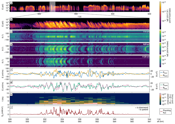
Fig 1
Some notes on this figure:
(1) Suggestion: consider adding the altitude of the payload to the x-axis of this figure to help contextualize measurements. This can be helpful for thinking about IAR's impact.
(2) Provide details for the filter used in the DC components.
(3) Suggestion: Separate out the E/B Field components into pairs on another panel. It's difficult to read on printed page otherwise.
(4) Should be differential energy flux instead of energy fluxWe thank the referee for these suggestions. We have revised Figure 1 and its caption as follow:
- The rocket altitude has been added to the x-axis labels.
- The caption and text now specify that the DC components were removed using a 6th order high-pass Butterworth filter with a cutoff frequency of 0.2 Hz.
- The electric- and magnetic-field components are now presented as paired components in separate panels.
- “Energy flux” has been corrected to “differential electron energy flux” in the figure caption and text.
L96
The mere existence of field aligned Poynting flux is insufficient to claim these are Alfven wave observations, and it is surprising no analysis using the wave data from Figure 1 was used for this purpose. For mostly downward-propagating, field-aligned Alfven waves near the ionosphere, the E/B ratio is expected to match the Alfven speed reasonably well. There even appears to be in-phase behavior between E_north and B_east in the data presented, which is typical. While a thorough analysis may be inappropriate for this paper, reporting the frequency range of the associated waves along with a brief E/B calculation adds necessary credibility.We agree that the field-aligned Poynting flux alone was insufficient to establish that the fluctuations were Alfvénic. A detailed study of Alfvén wave activity during the flight is left for a separate investigation by the collaborators, but we have added a short cross-spectral analysis of the perpendicular electric and magnetic fields. To avoid overloading the paper, the full analysis is presented in a new appendix and summarized in the overview. In the interval presented in Figure 1, the E/B ratio is found to be close to the estimated local Alfvén speed in the frequency band 1-8Hz, and the perpendicular field components show high coherence and cross-phases consistent with downward propagation in that same frequency band.
Fig 5
For the events in Fig 5 which are not shown in Fig 1, are they coincident with any other types of precipitation? Should they be thought of in the same way as those in Figure 1? This information is not given. Since the authors refer to the differences in plasma conditions along magnetic field lines throughout the paper often, this information would provide context on that point.Figure 5 has been redesigned to include an upper panel showing the differential electron energy-flux spectrogram over the entire interval containing the 29 analysed events. The interval of each selected event is marked on the spectrogram and connected to its corresponding source-altitude column in the lower panel. This allows the reader to assess the broader precipitation context of every event and to compare the events not included in Figure 1 with those shown there. Rocket altitude as well as MLAT/MLON of each event are also added to the x-axis labels.
L292 to L298, L308, L321, L409
For a linear IAW interpretation, variations in the plasma density along field lines or resonant source populations certainly affect the IAW phase speed and thereby the TOF fits, which is alluded to in this work. However, the variation in the wave perpendicular scales below 3km has also been shown by Tanaka 2005b (Fig 14 of that paper) to meaningfully modify the TOF polynomial fits. Additionally, in fig 1 of this paper the Poynting flux is well correlated with the flux intensity/peak energy of the electron dispersion (also consistent with Tanaka 2005b) and emphasizes that the waves themselves vary on the ~10 second spatial/temporal scales observed by this rocket. The author then considers dispersions over much of the several minutes of rocket flight in Fig 5, which increases the likelihood of the accelerating IAWs having different properties unless otherwise shown. Some words in the discussion or section 5.2 should acknowledge that variation in wave parameters between events can also modify TOF source altitude estimation instead of just differences of the plasma density, say.We agree that the original discussion placed too much emphasis on variations in plasma density. We have revised the relevant passages to state that both plasma conditions and wave properties may vary between events.
L371-393
While the assumption of matching IAW phase velocity with particle energy is understandable given the fitting method employed, it is important to specify sources of error by expanding upon L391-L393. Similiar to my previous comments, this fitting doesn't account for the parallel electrostatic potential of the IAW which accelerates electrons that are below V_A in parallel energy (but within the resonance window) and carries them over significant distances before being released. This point, at least, should be stated.We agree. We have expanded the discussion of the physical interpretation and limitations of the fitting method in Section 5.2. The revised manuscript now clarifies that the source altitudes should be interpreted as effective release altitudes rather than the locations at which acceleration begins/occurs, and that the matching of electron energy to v_A is a simplifying assumption. We explain that the parallel electric field defines a finite resonance window and that electrons in reality may leave the interaction at speeds below or above v_A.
--- Minor Comments/Technical Corrections ---
L30 Kletzing 1994 specifies the maximum energy of an IAW accelerated electrons in the laboratory frame as 2V_A - v_e, where v_e is the initial velocity of a resonant electron moving parallel to the wave.
The use of 2v_A in the preprint was a simplification. The revised manuscript gives the more complete upper velocity 2v_A – v_{\parallel0}, the initial parallel velocity of the resonant electron. We use this notation to avoid confusion with v_e , which denotes the electron thermal velocity elsewhere in the manuscript.
L31 There are multiple Kletzing 1994 references without identifiers, e.g. (a)/(b) between the two papers.
The two citations refer to distinct papers with different author lists:
- Kletzing, C. A.: Electron acceleration by kinetic Alfvén waves, Journal of Geophysical Research: Space Physics, 99, 11 095–11 103, https://doi.org/10.1029/94JA00345, 1994.
- Kletzing, C. A. and Torbert, R. B.: Electron time dispersion, Journal of Geophysical Research: Space Physics, 99, 2159–2172, https://doi.org/10.1029/93JA01745, 1994.
The first one is cited in the manuscript as “Kletzing, 1994” L31, L34 and L115, while the second one is cited as “Kletzing and Torbert, 1994” at L44. Because the author lists distinguish the citations in the text, identifiers should not be required. Every citation of these two papers has been rechecked to confirm that they point to the intended one.
L58 "with the aim to help improving" is difficult to read.
Rephrased to “[...] with the aim of improving [...]” in the revised manuscript.
L80, L395 It is not explicitly stated which flyer (low or high) data for Figure 1 comes only from. The text suggests its only the low flyer.
We have clarified in the overview (L80), the Figure 1 caption, Figure 5 caption and conclusion that the electron and field measurements used in this study all come from the low flyer.
L234 "...for some event to switch..." is awkward
This sentence has been revised.
L254 "to help" is awkward.
The awkward “to help” has been removed.
--- Other Remarks ---
While revising the manuscript, we
- Corrected a missing square root in the numerical implementation of the inertial Alfvén wave velocity (eq. 5). We re-ran all affected profiles and fits (Figures 6, 7 and quoted parameters). While this had some effect on the presented figures and exact values, the conclusions and outcomes of the paper remain unchanged.
- Replaced the linearized uncertainty visualization of Figure 7 (based on Jacobian covariance estimate) with a direct sampling of the fit-error landscape explored by the grid search. This gives a more accurate representation of the range of plasma and wave parameters compatible with the observations. The best-fit procedure and best-fit curve are unchanged. Only the “faint curves” and reported uncertainties are affected.
- Corrected an origin offset in the source altitudes of Figures 3 to 5. Field aligned path lengths were previously measured from the 100km starting altitude of our traced magnetic field lines rather than from the ground. We also decided to standardize the manuscript by reporting all source altitudes as geodetic heights (which differs from the field-aligned path length considered here by only approximately 1% as discussed in the first paragraph of Section 3). This is a difference from the preprint which was reporting source altitudes in path-length in Figures 3 to 5 and altitudes in geodetic heights in Figures 6 and 7. All source altitudes and altitudes now follow the same convention (geodetic height) throughout the manuscript and across figures. While this does not impact the previously submitted results, we hope this will make it easier for readers to follow the manuscript.
Citation: https://doi.org/10.5194/egusphere-2026-2126-AC1
-
AC1: 'Reply on RC1', Etienne Gavazzi, 24 Jul 2026
-
RC2: 'Comment on egusphere-2026-2126', Anonymous Referee #2, 11 Jun 2026
Review:
This article covers an interesting area of research. The investigation uses a high-quality dataset, discusses various methodologies for analyzing it, and applies them. It assesses different methodologies and demonstrates which method most likely provides the best information for describing the ionosphere density profile along the magnetic field line. It is a well-conducted scientific investigation that advances science and should be available to the community.
There are no major issues, and the articles can be published as is. These are suggested changes that can make the paper more impactful:
Figure 1: In text or at the bottom of the figure, indicate the change in the geomagnetic lat-long between 262s and 536s (this is the time period covered in Figure 5).
Line 145 and in the discussion: It is suggested that an instrument with high energy-time resolution is the best option for identifying the density altitude profile. However, when an observation is made close to the source region, the signature is easiest to see in the pitch-angle information. The text should acknowledge the importance of pitch-angle information so that future missions are designed with it in mind.
Line 145 and in the discussion: From an observational point of view, it is better to be far from the source to see DAW. The article does a great job of describing how to increase the accuracy when describing the source region (Figure 7); however, it could be valuable to balance the text by acknowledge having a standard instrument (with a similar resolution that was used in this study) at a slightly higher altitude on a satellite (which would degrade the accuracy) would instead provide more observations form any more different conditions. That is, this technique could be used to explore the altitude profiles of the ionosphere earthen (a) highly accurately with state-of-the-art instrumentation or (b) to get a sufficiently well-designed instrument that can observe the changes in the ionosphere over a long time. Both are valuable contributions to science.
Line 175, 255: Up-going particles are not used. This can be important information, improving the accuracy of the pitch-angle-time investigation. The manuscript should mention that and, hopefully, use it in future studies.
Line 205: remove 'despise'
Line 125: The first sentence indicates contrasting events, and the second sentence provides an example. However, the contrasting example appears several sentences later, making the text difficult to follow. Rearrange the paragraph so it is clear in the first or second sentence what the contrasting events/features are.
Figure 5 and line 300: Looking at the figure, a 30/60 second periodicity might be present. This periodicity could be of solar wind conditions outside the bow shock, which should be visible in magnetometer data, but it could be something else. Since the time periods in Figures 1 and 5 differ, it would be great if Figure 5 could add a second panel showing the energy spectrogram from 260s to 540s on top of the existing panel. It will also provide information on how easy/common the analyzed 29 events were. Adding the extra panel in Figure 5 would help to understand line 300.
Line 260-265: In this discussion, remind the reader of the altitude the rocket is moving at so that that information can be contrasted with the other observed speeds and altitudes. It is unclear if the results from the other investigations just reflect observations at different Geomagnetic latitudes and altitudes.
Line 320: This paragraph is good with an impact sentence at the end. However, it feels that this paragraph could benefit from a second impact sentence. Something, 'This is one of the few observation techniques that can provide density profiles of the ionosphere close to the critical inflection of the oxygen and hydrogen-dominant ionosphere, and allows the dynamics of the ionosphere to be investigated at aurora latitudes.'
Line 345: When describing the density profiles, rephrase it from 'low plasma densities' to describe the oxygen ionosphere profile with a small or a large scale height.
Line 350: When discussing cavities in the aurora region, it could be misinterpreted by readers. When satellites encounter a cavity, they observe a low-density region surrounded horizontally by higher densities. In Figure 6a, the vertical change in the density for the cavity profile is the same as the others. In the body of the text, it is therefore recommended not to use the word cavity and only use the word together with the reference. It is the combination of the small oxygen population's scale height and the small hydrogen component's scale height, relative to the magnetic field profile, that establishes the required Alfven speed profile for DAW waves to efficiently couple to the plasma, thereby creating the dispersed features as a result, as Figure 6 demonstrates.
Figure 7: The text does not mention the two bumps observed in Figure 7a. It is recommended that the manuscript address this, as it could be used for future high-accuracy observational investigations. It is a cool result.
Citation: https://doi.org/10.5194/egusphere-2026-2126-RC2 -
AC2: 'Reply on RC2', Etienne Gavazzi, 24 Jul 2026
We thank referee 2 for their positive assessment of the manuscript and for the constructive suggestions. We address each comment individually below.
Figure 1: In text or at the bottom of the figure, indicate the change in the geomagnetic lat-long between 262s and 536s (this is the time period covered in Figure 5).
Geomagnetic lat-long coordinates have been added to the x-axis labels of Figure 5.
Line 145 and in the discussion: It is suggested that an instrument with high energy-time resolution is the best option for identifying the density altitude profile. However, when an observation is made close to the source region, the signature is easiest to see in the pitch-angle information. The text should acknowledge the importance of pitch-angle information so that future missions are designed with it in mind.
We agree with the referee that the importance of pitch-angle information should be emphasized more clearly. In the revised manuscript, we now emphasize at the end of Section 5.2 that the proposed density-profile estimations rely on information extracted from the pitch-angle–time dispersions resolved across multiple energy channels and therefore require sufficient resolution in energy, time, and, importantly, pitch-angle. We hope that this more clearly motivates the inclusion of high-resolution pitch-angle capabilities in future missions.
Line 145 and in the discussion: From an observational point of view, it is better to be far from the source to see DAW. The article does a great job of describing how to increase the accuracy when describing the source region (Figure 7); however, it could be valuable to balance the text by acknowledge having a standard instrument (with a similar resolution that was used in this study) at a slightly higher altitude on a satellite (which would degrade the accuracy) would instead provide more observations form any more different conditions. That is, this technique could be used to explore the altitude profiles of the ionosphere earthen (a) highly accurately with state-of-the-art instrumentation or (b) to get a sufficiently well-designed instrument that can observe the changes in the ionosphere over a long time. Both are valuable contributions to science.
We thank the referee for highlighting this important observational trade-off. We have added a paragraph at the end of Section 5.2 discussing the two potential complementary observation strategies (sounding rockets and satellites).
Line 175, 255: Up-going particles are not used. This can be important information, improving the accuracy of the pitch-angle-time investigation. The manuscript should mention that and, hopefully, use it in future studies.
Good point. The dispersed signatures are also visible in higher-pitch-angle and up-going channels associated with mirroring electrons. However, the precipitation is strongly field-aligned, with decreasing flux with increasing pitch-angle, and our specific EESA instrument has channels with narrower angular widths near ±90, resulting in a lower signal-to-noise ratio degrading rather than improving the fits for the present dataset. For this reason, we excluded the near ±90 channels from our analysis. This is now explicitly stated in Section 3.2, and we note that future instruments with higher-sensitivity anodes may be able to exploit the additional information contained in the higher pitch-angles (including up-going) channels and therefore improve the source altitude constraints.
Line 205: remove 'despise'
We could not identify an occurrence of the word “despise” in the submitted preprint. We assume that the referee may have meant one of the occurrences of “despite”. We rechecked each occurrence of “despite” in the manuscript (L209, 286, 293, 299, 405 and 406) but found they were all used as intended. We therefore made no change in response to this comment.
Line 125: The first sentence indicates contrasting events, and the second sentence provides an example. However, the contrasting example appears several sentences later, making the text difficult to follow. Rearrange the paragraph so it is clear in the first or second sentence what the contrasting events/features are.
We assume that the referee intended to refer to the paragraph beginning around line 215 of the preprint, as this paragraph matches the description in the comment. We agree that the contrast between the events was introduced too late in the original paragraph. We have reorganized it so that the 338 s and 334 s events are identified as contrasting examples at the beginning, before describing each in more detail. This makes the text easier to read and follow.
Figure 5 and line 300: Looking at the figure, a 30/60 second periodicity might be present. This periodicity could be of solar wind conditions outside the bow shock, which should be visible in magnetometer data, but it could be something else. Since the time periods in Figures 1 and 5 differ, it would be great if Figure 5 could add a second panel showing the energy spectrogram from 260s to 540s on top of the existing panel. It will also provide information on how easy/common the analyzed 29 events were. Adding the extra panel in Figure 5 would help to understand line 300.
Figure 5 has been redesigned to include a top panel showing the energy spectrogram covering the full interval containing the 29 analysed events. The time span of each selected event is marked on the spectrogram and linked by connectors to the corresponding source-altitude column in the lower panel. This helps clarify the precipitation and temporal context of the events.
Line 260-265: In this discussion, remind the reader of the altitude the rocket is moving at so that that information can be contrasted with the other observed speeds and altitudes. It is unclear if the results from the other investigations just reflect observations at different Geomagnetic latitudes and altitudes.
The altitude (480-600km) and MLT (~13.5) during the observations of events included in Figure 5 are now stated in the discussion. This makes it easier to compare the results with the spacecraft altitudes and MLT of the other investigations presented in table 1.
Line 320: This paragraph is good with an impact sentence at the end. However, it feels that this paragraph could benefit from a second impact sentence. Something, 'This is one of the few observation techniques that can provide density profiles of the ionosphere close to the critical inflection of the oxygen and hydrogen-dominant ionosphere, and allows the dynamics of the ionosphere to be investigated at aurora latitudes.'
We thank the referee for this helpful suggestion. We have expanded the end of Section 5.2 to emphasize the broader potential of the technique. The revised manuscript now states that the method could become one of the few remote-sensing techniques capable of providing plasma density profiles near the transition between O+ and H+ dominated plasma. We link this with the modification above-mentioned about how satellite measurements could be used to investigate the spatial and temporal variability of this poorly sampled region of the auroral topside ionosphere.
Line 345: When describing the density profiles, rephrase it from 'low plasma densities' to describe the oxygen ionosphere profile with a small or a large scale height.
We agree that describing the profiles simply as having “low plasma densities” was somewhat imprecise. We have revised the discussion and conclusion to describe the relevant profiles in terms of their O+ scale heights. The source-altitude observations are now described as being most consistent with profiles having relatively small O+ scale heights, leading to a transition to H+ dominated plasma at lower altitudes.
Line 350: When discussing cavities in the aurora region, it could be misinterpreted by readers. When satellites encounter a cavity, they observe a low-density region surrounded horizontally by higher densities. In Figure 6a, the vertical change in the density for the cavity profile is the same as the others. In the body of the text, it is therefore recommended not to use the word cavity and only use the word together with the reference. It is the combination of the small oxygen population's scale height and the small hydrogen component's scale height, relative to the magnetic field profile, that establishes the required Alfven speed profile for DAW waves to efficiently couple to the plasma, thereby creating the dispersed features as a result, as Figure 6 demonstrates.
We thank the referee for highlighting this distinction. We have revised the manuscript to avoid using “density cavity” as a general description of the vertical density profiles. The term is now retained only when referring directly to the cited literature or when put into the context of satellite fly-by. Instead, we now describe our results primarily in terms of relatively small O+ scale heights and the resulting lower-altitude transition to H+ dominated plasma. We added a sentence explaining that, if neighboring field lines have larger O+ scale heights, measurements from a satellite traversing the region horizontally could be interpreted as a locally depleted auroral density cavity. This clarifies the separation between the inferred vertical profiles and the horizontally localized structures conventionally identified as cavities in satellite observations.
Figure 7: The text does not mention the two bumps observed in Figure 7a. It is recommended that the manuscript address this, as it could be used for future high-accuracy observational investigations. It is a cool result.
During revision, we identified a missing square root in the numerical implementation of the inertial Alfvén-wave velocity. After correcting the implementation and re-running the analysis, the double bump feature disappeared from Figure 7a.
The two bumps are still visible on a few other event fits. However, because the feature is no longer present in the example shown in Figure 7, we prefer not to interpret it in the present manuscript and leave it for future work.
--- Other Remarks ---
While revising the manuscript, we
- Corrected a missing square root in the numerical implementation of the inertial Alfvén wave velocity (eq. 5). We re-ran all affected profiles and fits (Figures 6, 7 and quoted parameters). While this had some effect on the presented figures and exact values, the conclusions and outcomes of the paper remain unchanged.
- Replaced the linearized uncertainty visualization of Figure 7 (based on Jacobian covariance estimate) with a direct sampling of the fit-error landscape explored by the grid search. This gives a more accurate representation of the range of plasma and wave parameters compatible with the observations. The best-fit procedure and best-fit curve are unchanged. Only the “faint curves” and reported uncertainties are affected.
- Corrected an origin offset in the source altitudes of Figures 3 to 5. Field aligned path lengths were previously measured from the 100km starting altitude of our traced magnetic field lines rather than from the ground. We also decided to standardize the manuscript by reporting all source altitudes as geodetic heights (which differs from the field-aligned path length considered here by only approximately 1% as discussed in the first paragraph of Section 3). This is a difference from the preprint which was reporting source altitudes in path-length in Figures 3 to 5 and altitudes in geodetic heights in Figures 6 and 7. All source altitudes and altitudes now follow the same convention (geodetic height) throughout the manuscript and across figures. While this does not impact the previously submitted results, we hope this will make it easier for readers to follow the manuscript.
Citation: https://doi.org/10.5194/egusphere-2026-2126-AC2
-
AC2: 'Reply on RC2', Etienne Gavazzi, 24 Jul 2026
Peer review completion


Interactive discussion
Status: closed
-
RC1: 'Comment on egusphere-2026-2126', Anonymous Referee #1, 08 Jun 2026
--- General Comments ---
This paper presents a dataset from the VISION-2 sounding rocket mission dealing with a pair of payloads that traveled southward into the dayside ionosphere. The analysis focuses on the many electron time dispersions observed by the low flyer's electrostatic analyzer, where historical time-of-flight methods are employed to estimate their source altitudes. The authors compare their predictions to the literature and those altitudes predicted by the inertial Alfven wave-particle acceleration process, developing a fitting method between the two in the process. The paper does not present a simulation/numerical model of the wave-particle acceleration process (which is known to occur many altitudes and depends upon the properties of the source plasma as well as accelerating waves) for their events, yet the authors acknowledges the limitations of their analysis while remaining reasonable. Although the electron dispersions, time of flight analysis and source mechanism for the dispersions are not new, the method of reverse-fitting dispersions to build up density profiles in a form of remote sensing is more novel and the succinct tabularization of the literature on this topic offer useful tools for further community discussion. I find this paper's core science and conclusions compelling for publication and believe it would be a great addition to the broader literature. However, minor caveats or considerations should be added to the paper to improve clarity regarding the limitations of the methods involved. In particular, the possible effects of the accelerating waves being different across their events as well as the accepted interpretation that resonant particles travel significant distances during IAW acceleration (as opposed to instantaneous release) complicate the interpretation presented, and should be acknowledged further.--- Specific Comments ---
L51/L115
While the limitations are known, the introduction or discussion section does not mention them. Such complications as variability in wave properties (poynting flux, wave scale, frequency, wave parallel potential), wave resonance bands or differences in source populations are not discussed/mentioned throughout.L79
The author references another paper to explain the particular pitch angle scheme which is supposed to explain how a 360deg/20bin = 18 deg/bin resolution detector can resolve 0-7.5degs in Figure 1. Unless the other referenced work is in hand, it is quite unclear how that is achieved. A very brief explanation of the scheme should be given in this manuscript.Fig 1
Some notes on this figure:
(1) Suggestion: consider adding the altitude of the payload to the x-axis of this figure to help contextualize measurements. This can be helpful for thinking about IAR's impact.
(2) Provide details for the filter used in the DC components.
(3) Suggestion: Separate out the E/B Field components into pairs on another panel. It's difficult to read on printed page otherwise.
(4) Should be differential energy flux instead of energy fluxL96
The mere existence of field aligned Poynting flux is insufficient to claim these are Alfven wave observations, and it is surprising no analysis using the wave data from Figure 1 was used for this purpose. For mostly downward-propagating, field-aligned Alfven waves near the ionosphere, the E/B ratio is expected to match the Alfven speed reasonably well. There even appears to be in-phase behavior between E_north and B_east in the data presented, which is typical. While a thorough analysis may be inappropriate for this paper, reporting the frequency range of the associated waves along with a brief E/B calculation adds necessary credibility.Fig 5
For the events in Fig 5 which are not shown in Fig 1, are they coincident with any other types of precipitation? Should they be thought of in the same way as those in Figure 1? This information is not given. Since the authors refer to the differences in plasma conditions along magnetic field lines throughout the paper often, this information would provide context on that point.L292 to L298, L308, L321, L409
For a linear IAW interpretation, variations in the plasma density along field lines or resonant source populations certainly affect the IAW phase speed and thereby the TOF fits, which is alluded to in this work. However, the variation in the wave perpendicular scales below 3km has also been shown by Tanaka 2005b (Fig 14 of that paper) to meaningfully modify the TOF polynomial fits. Additionally, in fig 1 of this paper the Poynting flux is well correlated with the flux intensity/peak energy of the electron dispersion (also consistent with Tanaka 2005b) and emphasizes that the waves themselves vary on the ~10 second spatial/temporal scales observed by this rocket. The author then considers dispersions over much of the several minutes of rocket flight in Fig 5, which increases the likelihood of the accelerating IAWs having different properties unless otherwise shown. Some words in the discussion or section 5.2 should acknowledge that variation in wave parameters between events can also modify TOF source altitude estimation instead of just differences of the plasma density, say.L371-393
While the assumption of matching IAW phase velocity with particle energy is understandable given the fitting method employed, it is important to specify sources of error by expanding upon L391-L393. Similiar to my previous comments, this fitting doesn't account for the parallel electrostatic potential of the IAW which accelerates electrons that are below V_A in parallel energy (but within the resonance window) and carries them over significant distances before being released. This point, at least, should be stated.--- Minor Comments/Technical Corrections ---
L30 Kletzing 1994 specifies the maximum energy of an IAW accelerated electrons in the laboratory frame as 2V_A - v_e, where v_e is the initial velocity of a resonant electron moving parallel to the wave.
L31 There are multiple Kletzing 1994 references without identifiers, e.g. (a)/(b) between the two papers.
L58 "with the aim to help improving" is difficult to read.
L80, L395 It is not explicitly stated which flyer (low or high) data for Figure 1 comes only from. The text suggests its only the low flyer.
L234 "...for some event to switch..." is awkward
L254 "to help" is awkward.
Citation: https://doi.org/10.5194/egusphere-2026-2126-RC1 -
AC1: 'Reply on RC1', Etienne Gavazzi, 24 Jul 2026
We thank referee 1 for their positive assessment of the manuscript and for the constructive comments. We agree that the original manuscript did not sufficiently discuss the possible (and likely) variability of the accelerating waves across events. We also agree that the physical description of particle acceleration by the wave could be improved, by mentioning that the particles can travel with the wave and be accelerated over significant distances, and that as such the inferred “source altitudes” should be interpreted as effective “release altitudes” at which the particles leave the resonant interaction.
We believe that these clarifications strengthen both the manuscript and the interpretation of the results.
--- Specific Comments ---
L51/L115
While the limitations are known, the introduction or discussion section does not mention them. Such complications as variability in wave properties (poynting flux, wave scale, frequency, wave parallel potential), wave resonance bands or differences in source populations are not discussed/mentioned throughout.We have expanded the manuscript in several places. At the beginning of Section 3, we now clarify that resonant electrons can be transported and progressively energized over substantial distances and that the inferred “source altitudes” should therefore be interpreted as effective release altitudes. In Section 5.2, we now explicitly acknowledge that the morphology of the dispersions can also depend on wave properties as well as on the density and temperature of the source electron population. We have added in several places that differences between events cannot be attributed uniquely to variations in the background plasma density but also to wave parameters. We also clarify that the present fitting procedure constrains only the density-profile parameters and perpendicular wave scale because these are the parameters that enter the inertial Alfvén velocity equation directly.
L79
The author references another paper to explain the particular pitch angle scheme which is supposed to explain how a 360deg/20bin = 18 deg/bin resolution detector can resolve 0-7.5degs in Figure 1. Unless the other referenced work is in hand, it is quite unclear how that is achieved. A very brief explanation of the scheme should be given in this manuscript.Good point. The EESA instrument has pitch angle channels with different angular widths. We have clarified this in the overview around L79 and added an appendix table listing the central pitch-angle direction and angular width of every channel.
Fig 1
Some notes on this figure:
(1) Suggestion: consider adding the altitude of the payload to the x-axis of this figure to help contextualize measurements. This can be helpful for thinking about IAR's impact.
(2) Provide details for the filter used in the DC components.
(3) Suggestion: Separate out the E/B Field components into pairs on another panel. It's difficult to read on printed page otherwise.
(4) Should be differential energy flux instead of energy fluxWe thank the referee for these suggestions. We have revised Figure 1 and its caption as follow:
- The rocket altitude has been added to the x-axis labels.
- The caption and text now specify that the DC components were removed using a 6th order high-pass Butterworth filter with a cutoff frequency of 0.2 Hz.
- The electric- and magnetic-field components are now presented as paired components in separate panels.
- “Energy flux” has been corrected to “differential electron energy flux” in the figure caption and text.
L96
The mere existence of field aligned Poynting flux is insufficient to claim these are Alfven wave observations, and it is surprising no analysis using the wave data from Figure 1 was used for this purpose. For mostly downward-propagating, field-aligned Alfven waves near the ionosphere, the E/B ratio is expected to match the Alfven speed reasonably well. There even appears to be in-phase behavior between E_north and B_east in the data presented, which is typical. While a thorough analysis may be inappropriate for this paper, reporting the frequency range of the associated waves along with a brief E/B calculation adds necessary credibility.We agree that the field-aligned Poynting flux alone was insufficient to establish that the fluctuations were Alfvénic. A detailed study of Alfvén wave activity during the flight is left for a separate investigation by the collaborators, but we have added a short cross-spectral analysis of the perpendicular electric and magnetic fields. To avoid overloading the paper, the full analysis is presented in a new appendix and summarized in the overview. In the interval presented in Figure 1, the E/B ratio is found to be close to the estimated local Alfvén speed in the frequency band 1-8Hz, and the perpendicular field components show high coherence and cross-phases consistent with downward propagation in that same frequency band.
Fig 5
For the events in Fig 5 which are not shown in Fig 1, are they coincident with any other types of precipitation? Should they be thought of in the same way as those in Figure 1? This information is not given. Since the authors refer to the differences in plasma conditions along magnetic field lines throughout the paper often, this information would provide context on that point.Figure 5 has been redesigned to include an upper panel showing the differential electron energy-flux spectrogram over the entire interval containing the 29 analysed events. The interval of each selected event is marked on the spectrogram and connected to its corresponding source-altitude column in the lower panel. This allows the reader to assess the broader precipitation context of every event and to compare the events not included in Figure 1 with those shown there. Rocket altitude as well as MLAT/MLON of each event are also added to the x-axis labels.
L292 to L298, L308, L321, L409
For a linear IAW interpretation, variations in the plasma density along field lines or resonant source populations certainly affect the IAW phase speed and thereby the TOF fits, which is alluded to in this work. However, the variation in the wave perpendicular scales below 3km has also been shown by Tanaka 2005b (Fig 14 of that paper) to meaningfully modify the TOF polynomial fits. Additionally, in fig 1 of this paper the Poynting flux is well correlated with the flux intensity/peak energy of the electron dispersion (also consistent with Tanaka 2005b) and emphasizes that the waves themselves vary on the ~10 second spatial/temporal scales observed by this rocket. The author then considers dispersions over much of the several minutes of rocket flight in Fig 5, which increases the likelihood of the accelerating IAWs having different properties unless otherwise shown. Some words in the discussion or section 5.2 should acknowledge that variation in wave parameters between events can also modify TOF source altitude estimation instead of just differences of the plasma density, say.We agree that the original discussion placed too much emphasis on variations in plasma density. We have revised the relevant passages to state that both plasma conditions and wave properties may vary between events.
L371-393
While the assumption of matching IAW phase velocity with particle energy is understandable given the fitting method employed, it is important to specify sources of error by expanding upon L391-L393. Similiar to my previous comments, this fitting doesn't account for the parallel electrostatic potential of the IAW which accelerates electrons that are below V_A in parallel energy (but within the resonance window) and carries them over significant distances before being released. This point, at least, should be stated.We agree. We have expanded the discussion of the physical interpretation and limitations of the fitting method in Section 5.2. The revised manuscript now clarifies that the source altitudes should be interpreted as effective release altitudes rather than the locations at which acceleration begins/occurs, and that the matching of electron energy to v_A is a simplifying assumption. We explain that the parallel electric field defines a finite resonance window and that electrons in reality may leave the interaction at speeds below or above v_A.
--- Minor Comments/Technical Corrections ---
L30 Kletzing 1994 specifies the maximum energy of an IAW accelerated electrons in the laboratory frame as 2V_A - v_e, where v_e is the initial velocity of a resonant electron moving parallel to the wave.
The use of 2v_A in the preprint was a simplification. The revised manuscript gives the more complete upper velocity 2v_A – v_{\parallel0}, the initial parallel velocity of the resonant electron. We use this notation to avoid confusion with v_e , which denotes the electron thermal velocity elsewhere in the manuscript.
L31 There are multiple Kletzing 1994 references without identifiers, e.g. (a)/(b) between the two papers.
The two citations refer to distinct papers with different author lists:
- Kletzing, C. A.: Electron acceleration by kinetic Alfvén waves, Journal of Geophysical Research: Space Physics, 99, 11 095–11 103, https://doi.org/10.1029/94JA00345, 1994.
- Kletzing, C. A. and Torbert, R. B.: Electron time dispersion, Journal of Geophysical Research: Space Physics, 99, 2159–2172, https://doi.org/10.1029/93JA01745, 1994.
The first one is cited in the manuscript as “Kletzing, 1994” L31, L34 and L115, while the second one is cited as “Kletzing and Torbert, 1994” at L44. Because the author lists distinguish the citations in the text, identifiers should not be required. Every citation of these two papers has been rechecked to confirm that they point to the intended one.
L58 "with the aim to help improving" is difficult to read.
Rephrased to “[...] with the aim of improving [...]” in the revised manuscript.
L80, L395 It is not explicitly stated which flyer (low or high) data for Figure 1 comes only from. The text suggests its only the low flyer.
We have clarified in the overview (L80), the Figure 1 caption, Figure 5 caption and conclusion that the electron and field measurements used in this study all come from the low flyer.
L234 "...for some event to switch..." is awkward
This sentence has been revised.
L254 "to help" is awkward.
The awkward “to help” has been removed.
--- Other Remarks ---
While revising the manuscript, we
- Corrected a missing square root in the numerical implementation of the inertial Alfvén wave velocity (eq. 5). We re-ran all affected profiles and fits (Figures 6, 7 and quoted parameters). While this had some effect on the presented figures and exact values, the conclusions and outcomes of the paper remain unchanged.
- Replaced the linearized uncertainty visualization of Figure 7 (based on Jacobian covariance estimate) with a direct sampling of the fit-error landscape explored by the grid search. This gives a more accurate representation of the range of plasma and wave parameters compatible with the observations. The best-fit procedure and best-fit curve are unchanged. Only the “faint curves” and reported uncertainties are affected.
- Corrected an origin offset in the source altitudes of Figures 3 to 5. Field aligned path lengths were previously measured from the 100km starting altitude of our traced magnetic field lines rather than from the ground. We also decided to standardize the manuscript by reporting all source altitudes as geodetic heights (which differs from the field-aligned path length considered here by only approximately 1% as discussed in the first paragraph of Section 3). This is a difference from the preprint which was reporting source altitudes in path-length in Figures 3 to 5 and altitudes in geodetic heights in Figures 6 and 7. All source altitudes and altitudes now follow the same convention (geodetic height) throughout the manuscript and across figures. While this does not impact the previously submitted results, we hope this will make it easier for readers to follow the manuscript.
Citation: https://doi.org/10.5194/egusphere-2026-2126-AC1
-
AC1: 'Reply on RC1', Etienne Gavazzi, 24 Jul 2026
-
RC2: 'Comment on egusphere-2026-2126', Anonymous Referee #2, 11 Jun 2026
Review:
This article covers an interesting area of research. The investigation uses a high-quality dataset, discusses various methodologies for analyzing it, and applies them. It assesses different methodologies and demonstrates which method most likely provides the best information for describing the ionosphere density profile along the magnetic field line. It is a well-conducted scientific investigation that advances science and should be available to the community.
There are no major issues, and the articles can be published as is. These are suggested changes that can make the paper more impactful:
Figure 1: In text or at the bottom of the figure, indicate the change in the geomagnetic lat-long between 262s and 536s (this is the time period covered in Figure 5).
Line 145 and in the discussion: It is suggested that an instrument with high energy-time resolution is the best option for identifying the density altitude profile. However, when an observation is made close to the source region, the signature is easiest to see in the pitch-angle information. The text should acknowledge the importance of pitch-angle information so that future missions are designed with it in mind.
Line 145 and in the discussion: From an observational point of view, it is better to be far from the source to see DAW. The article does a great job of describing how to increase the accuracy when describing the source region (Figure 7); however, it could be valuable to balance the text by acknowledge having a standard instrument (with a similar resolution that was used in this study) at a slightly higher altitude on a satellite (which would degrade the accuracy) would instead provide more observations form any more different conditions. That is, this technique could be used to explore the altitude profiles of the ionosphere earthen (a) highly accurately with state-of-the-art instrumentation or (b) to get a sufficiently well-designed instrument that can observe the changes in the ionosphere over a long time. Both are valuable contributions to science.
Line 175, 255: Up-going particles are not used. This can be important information, improving the accuracy of the pitch-angle-time investigation. The manuscript should mention that and, hopefully, use it in future studies.
Line 205: remove 'despise'
Line 125: The first sentence indicates contrasting events, and the second sentence provides an example. However, the contrasting example appears several sentences later, making the text difficult to follow. Rearrange the paragraph so it is clear in the first or second sentence what the contrasting events/features are.
Figure 5 and line 300: Looking at the figure, a 30/60 second periodicity might be present. This periodicity could be of solar wind conditions outside the bow shock, which should be visible in magnetometer data, but it could be something else. Since the time periods in Figures 1 and 5 differ, it would be great if Figure 5 could add a second panel showing the energy spectrogram from 260s to 540s on top of the existing panel. It will also provide information on how easy/common the analyzed 29 events were. Adding the extra panel in Figure 5 would help to understand line 300.
Line 260-265: In this discussion, remind the reader of the altitude the rocket is moving at so that that information can be contrasted with the other observed speeds and altitudes. It is unclear if the results from the other investigations just reflect observations at different Geomagnetic latitudes and altitudes.
Line 320: This paragraph is good with an impact sentence at the end. However, it feels that this paragraph could benefit from a second impact sentence. Something, 'This is one of the few observation techniques that can provide density profiles of the ionosphere close to the critical inflection of the oxygen and hydrogen-dominant ionosphere, and allows the dynamics of the ionosphere to be investigated at aurora latitudes.'
Line 345: When describing the density profiles, rephrase it from 'low plasma densities' to describe the oxygen ionosphere profile with a small or a large scale height.
Line 350: When discussing cavities in the aurora region, it could be misinterpreted by readers. When satellites encounter a cavity, they observe a low-density region surrounded horizontally by higher densities. In Figure 6a, the vertical change in the density for the cavity profile is the same as the others. In the body of the text, it is therefore recommended not to use the word cavity and only use the word together with the reference. It is the combination of the small oxygen population's scale height and the small hydrogen component's scale height, relative to the magnetic field profile, that establishes the required Alfven speed profile for DAW waves to efficiently couple to the plasma, thereby creating the dispersed features as a result, as Figure 6 demonstrates.
Figure 7: The text does not mention the two bumps observed in Figure 7a. It is recommended that the manuscript address this, as it could be used for future high-accuracy observational investigations. It is a cool result.
Citation: https://doi.org/10.5194/egusphere-2026-2126-RC2 -
AC2: 'Reply on RC2', Etienne Gavazzi, 24 Jul 2026
We thank referee 2 for their positive assessment of the manuscript and for the constructive suggestions. We address each comment individually below.
Figure 1: In text or at the bottom of the figure, indicate the change in the geomagnetic lat-long between 262s and 536s (this is the time period covered in Figure 5).
Geomagnetic lat-long coordinates have been added to the x-axis labels of Figure 5.
Line 145 and in the discussion: It is suggested that an instrument with high energy-time resolution is the best option for identifying the density altitude profile. However, when an observation is made close to the source region, the signature is easiest to see in the pitch-angle information. The text should acknowledge the importance of pitch-angle information so that future missions are designed with it in mind.
We agree with the referee that the importance of pitch-angle information should be emphasized more clearly. In the revised manuscript, we now emphasize at the end of Section 5.2 that the proposed density-profile estimations rely on information extracted from the pitch-angle–time dispersions resolved across multiple energy channels and therefore require sufficient resolution in energy, time, and, importantly, pitch-angle. We hope that this more clearly motivates the inclusion of high-resolution pitch-angle capabilities in future missions.
Line 145 and in the discussion: From an observational point of view, it is better to be far from the source to see DAW. The article does a great job of describing how to increase the accuracy when describing the source region (Figure 7); however, it could be valuable to balance the text by acknowledge having a standard instrument (with a similar resolution that was used in this study) at a slightly higher altitude on a satellite (which would degrade the accuracy) would instead provide more observations form any more different conditions. That is, this technique could be used to explore the altitude profiles of the ionosphere earthen (a) highly accurately with state-of-the-art instrumentation or (b) to get a sufficiently well-designed instrument that can observe the changes in the ionosphere over a long time. Both are valuable contributions to science.
We thank the referee for highlighting this important observational trade-off. We have added a paragraph at the end of Section 5.2 discussing the two potential complementary observation strategies (sounding rockets and satellites).
Line 175, 255: Up-going particles are not used. This can be important information, improving the accuracy of the pitch-angle-time investigation. The manuscript should mention that and, hopefully, use it in future studies.
Good point. The dispersed signatures are also visible in higher-pitch-angle and up-going channels associated with mirroring electrons. However, the precipitation is strongly field-aligned, with decreasing flux with increasing pitch-angle, and our specific EESA instrument has channels with narrower angular widths near ±90, resulting in a lower signal-to-noise ratio degrading rather than improving the fits for the present dataset. For this reason, we excluded the near ±90 channels from our analysis. This is now explicitly stated in Section 3.2, and we note that future instruments with higher-sensitivity anodes may be able to exploit the additional information contained in the higher pitch-angles (including up-going) channels and therefore improve the source altitude constraints.
Line 205: remove 'despise'
We could not identify an occurrence of the word “despise” in the submitted preprint. We assume that the referee may have meant one of the occurrences of “despite”. We rechecked each occurrence of “despite” in the manuscript (L209, 286, 293, 299, 405 and 406) but found they were all used as intended. We therefore made no change in response to this comment.
Line 125: The first sentence indicates contrasting events, and the second sentence provides an example. However, the contrasting example appears several sentences later, making the text difficult to follow. Rearrange the paragraph so it is clear in the first or second sentence what the contrasting events/features are.
We assume that the referee intended to refer to the paragraph beginning around line 215 of the preprint, as this paragraph matches the description in the comment. We agree that the contrast between the events was introduced too late in the original paragraph. We have reorganized it so that the 338 s and 334 s events are identified as contrasting examples at the beginning, before describing each in more detail. This makes the text easier to read and follow.
Figure 5 and line 300: Looking at the figure, a 30/60 second periodicity might be present. This periodicity could be of solar wind conditions outside the bow shock, which should be visible in magnetometer data, but it could be something else. Since the time periods in Figures 1 and 5 differ, it would be great if Figure 5 could add a second panel showing the energy spectrogram from 260s to 540s on top of the existing panel. It will also provide information on how easy/common the analyzed 29 events were. Adding the extra panel in Figure 5 would help to understand line 300.
Figure 5 has been redesigned to include a top panel showing the energy spectrogram covering the full interval containing the 29 analysed events. The time span of each selected event is marked on the spectrogram and linked by connectors to the corresponding source-altitude column in the lower panel. This helps clarify the precipitation and temporal context of the events.
Line 260-265: In this discussion, remind the reader of the altitude the rocket is moving at so that that information can be contrasted with the other observed speeds and altitudes. It is unclear if the results from the other investigations just reflect observations at different Geomagnetic latitudes and altitudes.
The altitude (480-600km) and MLT (~13.5) during the observations of events included in Figure 5 are now stated in the discussion. This makes it easier to compare the results with the spacecraft altitudes and MLT of the other investigations presented in table 1.
Line 320: This paragraph is good with an impact sentence at the end. However, it feels that this paragraph could benefit from a second impact sentence. Something, 'This is one of the few observation techniques that can provide density profiles of the ionosphere close to the critical inflection of the oxygen and hydrogen-dominant ionosphere, and allows the dynamics of the ionosphere to be investigated at aurora latitudes.'
We thank the referee for this helpful suggestion. We have expanded the end of Section 5.2 to emphasize the broader potential of the technique. The revised manuscript now states that the method could become one of the few remote-sensing techniques capable of providing plasma density profiles near the transition between O+ and H+ dominated plasma. We link this with the modification above-mentioned about how satellite measurements could be used to investigate the spatial and temporal variability of this poorly sampled region of the auroral topside ionosphere.
Line 345: When describing the density profiles, rephrase it from 'low plasma densities' to describe the oxygen ionosphere profile with a small or a large scale height.
We agree that describing the profiles simply as having “low plasma densities” was somewhat imprecise. We have revised the discussion and conclusion to describe the relevant profiles in terms of their O+ scale heights. The source-altitude observations are now described as being most consistent with profiles having relatively small O+ scale heights, leading to a transition to H+ dominated plasma at lower altitudes.
Line 350: When discussing cavities in the aurora region, it could be misinterpreted by readers. When satellites encounter a cavity, they observe a low-density region surrounded horizontally by higher densities. In Figure 6a, the vertical change in the density for the cavity profile is the same as the others. In the body of the text, it is therefore recommended not to use the word cavity and only use the word together with the reference. It is the combination of the small oxygen population's scale height and the small hydrogen component's scale height, relative to the magnetic field profile, that establishes the required Alfven speed profile for DAW waves to efficiently couple to the plasma, thereby creating the dispersed features as a result, as Figure 6 demonstrates.
We thank the referee for highlighting this distinction. We have revised the manuscript to avoid using “density cavity” as a general description of the vertical density profiles. The term is now retained only when referring directly to the cited literature or when put into the context of satellite fly-by. Instead, we now describe our results primarily in terms of relatively small O+ scale heights and the resulting lower-altitude transition to H+ dominated plasma. We added a sentence explaining that, if neighboring field lines have larger O+ scale heights, measurements from a satellite traversing the region horizontally could be interpreted as a locally depleted auroral density cavity. This clarifies the separation between the inferred vertical profiles and the horizontally localized structures conventionally identified as cavities in satellite observations.
Figure 7: The text does not mention the two bumps observed in Figure 7a. It is recommended that the manuscript address this, as it could be used for future high-accuracy observational investigations. It is a cool result.
During revision, we identified a missing square root in the numerical implementation of the inertial Alfvén-wave velocity. After correcting the implementation and re-running the analysis, the double bump feature disappeared from Figure 7a.
The two bumps are still visible on a few other event fits. However, because the feature is no longer present in the example shown in Figure 7, we prefer not to interpret it in the present manuscript and leave it for future work.
--- Other Remarks ---
While revising the manuscript, we
- Corrected a missing square root in the numerical implementation of the inertial Alfvén wave velocity (eq. 5). We re-ran all affected profiles and fits (Figures 6, 7 and quoted parameters). While this had some effect on the presented figures and exact values, the conclusions and outcomes of the paper remain unchanged.
- Replaced the linearized uncertainty visualization of Figure 7 (based on Jacobian covariance estimate) with a direct sampling of the fit-error landscape explored by the grid search. This gives a more accurate representation of the range of plasma and wave parameters compatible with the observations. The best-fit procedure and best-fit curve are unchanged. Only the “faint curves” and reported uncertainties are affected.
- Corrected an origin offset in the source altitudes of Figures 3 to 5. Field aligned path lengths were previously measured from the 100km starting altitude of our traced magnetic field lines rather than from the ground. We also decided to standardize the manuscript by reporting all source altitudes as geodetic heights (which differs from the field-aligned path length considered here by only approximately 1% as discussed in the first paragraph of Section 3). This is a difference from the preprint which was reporting source altitudes in path-length in Figures 3 to 5 and altitudes in geodetic heights in Figures 6 and 7. All source altitudes and altitudes now follow the same convention (geodetic height) throughout the manuscript and across figures. While this does not impact the previously submitted results, we hope this will make it easier for readers to follow the manuscript.
Citation: https://doi.org/10.5194/egusphere-2026-2126-AC2
-
AC2: 'Reply on RC2', Etienne Gavazzi, 24 Jul 2026
Peer review completion
Journal article(s) based on this preprint
Viewed
| HTML | XML | Total | BibTeX | EndNote | |
|---|---|---|---|---|---|
| 257 | 159 | 35 | 451 | 36 | 34 |
- HTML: 257
- PDF: 159
- XML: 35
- Total: 451
- BibTeX: 36
- EndNote: 34
Viewed (geographical distribution)
| Country | # | Views | % |
|---|
| Total: | 0 |
| HTML: | 0 |
| PDF: | 0 |
| XML: | 0 |
- 1

Andres Spicher
Björn Gustavsson
Juha Vierinen
James Clemmons
Robert Pfaff
Douglas Rowland
The requested preprint has a corresponding peer-reviewed final revised paper. You are encouraged to refer to the final revised version.
- Preprint
(7948 KB) - Metadata XML
--- General Comments ---
This paper presents a dataset from the VISION-2 sounding rocket mission dealing with a pair of payloads that traveled southward into the dayside ionosphere. The analysis focuses on the many electron time dispersions observed by the low flyer's electrostatic analyzer, where historical time-of-flight methods are employed to estimate their source altitudes. The authors compare their predictions to the literature and those altitudes predicted by the inertial Alfven wave-particle acceleration process, developing a fitting method between the two in the process. The paper does not present a simulation/numerical model of the wave-particle acceleration process (which is known to occur many altitudes and depends upon the properties of the source plasma as well as accelerating waves) for their events, yet the authors acknowledges the limitations of their analysis while remaining reasonable. Although the electron dispersions, time of flight analysis and source mechanism for the dispersions are not new, the method of reverse-fitting dispersions to build up density profiles in a form of remote sensing is more novel and the succinct tabularization of the literature on this topic offer useful tools for further community discussion. I find this paper's core science and conclusions compelling for publication and believe it would be a great addition to the broader literature. However, minor caveats or considerations should be added to the paper to improve clarity regarding the limitations of the methods involved. In particular, the possible effects of the accelerating waves being different across their events as well as the accepted interpretation that resonant particles travel significant distances during IAW acceleration (as opposed to instantaneous release) complicate the interpretation presented, and should be acknowledged further.
--- Specific Comments ---
L51/L115
While the limitations are known, the introduction or discussion section does not mention them. Such complications as variability in wave properties (poynting flux, wave scale, frequency, wave parallel potential), wave resonance bands or differences in source populations are not discussed/mentioned throughout.
L79
The author references another paper to explain the particular pitch angle scheme which is supposed to explain how a 360deg/20bin = 18 deg/bin resolution detector can resolve 0-7.5degs in Figure 1. Unless the other referenced work is in hand, it is quite unclear how that is achieved. A very brief explanation of the scheme should be given in this manuscript.
Fig 1
Some notes on this figure:
(1) Suggestion: consider adding the altitude of the payload to the x-axis of this figure to help contextualize measurements. This can be helpful for thinking about IAR's impact.
(2) Provide details for the filter used in the DC components.
(3) Suggestion: Separate out the E/B Field components into pairs on another panel. It's difficult to read on printed page otherwise.
(4) Should be differential energy flux instead of energy flux
L96
The mere existence of field aligned Poynting flux is insufficient to claim these are Alfven wave observations, and it is surprising no analysis using the wave data from Figure 1 was used for this purpose. For mostly downward-propagating, field-aligned Alfven waves near the ionosphere, the E/B ratio is expected to match the Alfven speed reasonably well. There even appears to be in-phase behavior between E_north and B_east in the data presented, which is typical. While a thorough analysis may be inappropriate for this paper, reporting the frequency range of the associated waves along with a brief E/B calculation adds necessary credibility.
Fig 5
For the events in Fig 5 which are not shown in Fig 1, are they coincident with any other types of precipitation? Should they be thought of in the same way as those in Figure 1? This information is not given. Since the authors refer to the differences in plasma conditions along magnetic field lines throughout the paper often, this information would provide context on that point.
L292 to L298, L308, L321, L409
For a linear IAW interpretation, variations in the plasma density along field lines or resonant source populations certainly affect the IAW phase speed and thereby the TOF fits, which is alluded to in this work. However, the variation in the wave perpendicular scales below 3km has also been shown by Tanaka 2005b (Fig 14 of that paper) to meaningfully modify the TOF polynomial fits. Additionally, in fig 1 of this paper the Poynting flux is well correlated with the flux intensity/peak energy of the electron dispersion (also consistent with Tanaka 2005b) and emphasizes that the waves themselves vary on the ~10 second spatial/temporal scales observed by this rocket. The author then considers dispersions over much of the several minutes of rocket flight in Fig 5, which increases the likelihood of the accelerating IAWs having different properties unless otherwise shown. Some words in the discussion or section 5.2 should acknowledge that variation in wave parameters between events can also modify TOF source altitude estimation instead of just differences of the plasma density, say.
L371-393
While the assumption of matching IAW phase velocity with particle energy is understandable given the fitting method employed, it is important to specify sources of error by expanding upon L391-L393. Similiar to my previous comments, this fitting doesn't account for the parallel electrostatic potential of the IAW which accelerates electrons that are below V_A in parallel energy (but within the resonance window) and carries them over significant distances before being released. This point, at least, should be stated.
--- Minor Comments/Technical Corrections ---
L30 Kletzing 1994 specifies the maximum energy of an IAW accelerated electrons in the laboratory frame as 2V_A - v_e, where v_e is the initial velocity of a resonant electron moving parallel to the wave.
L31 There are multiple Kletzing 1994 references without identifiers, e.g. (a)/(b) between the two papers.
L58 "with the aim to help improving" is difficult to read.
L80, L395 It is not explicitly stated which flyer (low or high) data for Figure 1 comes only from. The text suggests its only the low flyer.
L234 "...for some event to switch..." is awkward
L254 "to help" is awkward.