
the Creative Commons Attribution 4.0 License.
the Creative Commons Attribution 4.0 License.
 | 18 May 2026
METEORv1.6: Spatial climate variability and integrated impact emulation
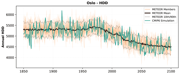
Abstract. Climate impact assessment increasingly requires spatially explicit projections with realistic temporal variability at sub-annual resolution. METEORv1.6 extends the established METEOR spatial multi-timescale, multi-forcer climate emulation framework with two major capabilities: (1) a monthly climate variability model that generates realistic sub-annual climate sequences with seasonal cycles and inter-annual variability, enabling the generation of ensemble projections and (2) a modular impact assessment framework that translates climate projections into impact metrics. The monthly climate model represents seasonal harmonics and noise, while preserving covariance structures from the source model. Seasonal cycles are represented through harmonic analysis with temperature-dependent parameterization, enabling non-stationary simulation of seasonal timing shifts under warming. Principal Component Analysis is used to decompose monthly anomalies into spatial modes, then their temporal evolution and climate variability is modeled using Vector Autoregressive with eXogenous variables (VARX) processes. The impact assessment framework provides a standardized interface for ensemble processing and uncertainty quantification through a modular system of impact calculators. The initial case implementation includes heating and cooling degree days calculations which are key drivers in estimating energy sector demand, demonstrating ensemble-based uncertainty propagation from climate projections to impact metrics. Validation against CMIP6 data demonstrates that METEORv1.6 accurately reproduces statistical properties of monthly climate variability for a range of future scenarios when trained on a single scenario from an Earth System Model (together with a CO2 quadrupling idealized experiment). The integrated impact framework enables rapid generation of probabilistic climate risk assessments suitable for sectoral applications, bridging the gap between global climate projections and local decision-making needs. The open-source implementation supports broad adoption and continued expansion to additional impact domains.
-
Notice on discussion status
The requested preprint has a corresponding peer-reviewed final revised paper. You are encouraged to refer to the final revised version.
-
Preprint
(3533 KB)
-
Supplement
(1680 KB)
-
The requested preprint has a corresponding peer-reviewed final revised paper. You are encouraged to refer to the final revised version.
- Preprint
(3533 KB) - Metadata XML
-
Supplement
(1680 KB) - BibTeX
- EndNote
- Final revised paper


Journal article(s) based on this preprint
Interactive discussion
Status: closed
-
CEC1: 'Comment on egusphere-2026-2029 - No compliance with the policy of the journal', Juan Antonio Añel, 21 Jun 2026
-
CC1: 'Reply on CEC1', Marit Sandstad, 21 Jun 2026
Dear Juan A. Añel,
All CMIP6 data are available through the Earth System Grid Federation (ESGF; Cinquini et al., 2014) or via the zarrstore google-api (https://storage.googleapis.com/cmip6/cmip6-zarr-consolidated-stores.csv). As was described in the description paper for the first version of METEOR (Sandstad et. al 2025), METEOR includes software that directly pulls and processes data from the zarrstore google-api to do its training, so the model can be retrained an run with no manual outside of METEOR data download from a separate repository.
We are very sorry if this was not clear from our current Data Availability section and we will update that shortly.
Hope that clarifies the points and will be enough to show that we are in compliance with the journals "Code and Data policy"
Best regards,
Marit Sandstad
Cinquini, L., Crichton, D., Mattmann, C., Harney, J., Shipman, G., Wang, F., Ananthakrishnan, R., Miller, N., Denvil, S., Morgan, M., Pobre, Z., Bell, G. M., Doutriaux, C., Drach, R., Williams, D., Kershaw, P., Pascoe, S., Gonzalez, E., Fiore, S., and Schweitzer, R.: The Earth System Grid Federation: An open infrastructure for access to distributed geospatial data, Future Gener. Comput. Syst., 36, 400–417, https://esgf-node.llnl.gov
Sandstad, M., Steinert, N. J., Baur, S., and Sanderson, B. M.: METEORv1.0.1: a novel framework for emulating multi-timescale regional climate responses, Geosci. Model Dev., 18, 8269–8312, https://doi.org/10.5194/gmd-18-8269-2025, 2025.
Citation: https://doi.org/10.5194/egusphere-2026-2029-CC1 -
CEC2: 'Reply on CC1', Juan Antonio Añel, 21 Jun 2026
Dear authors,
Many thanks for the quick reply. Unfortunately, we can not accept that the data used in the work presented are stored in googleapis.com. Namely:
- It does not appear to have a published policy for data preservation over many years or decades (some flexibility exists over the precise length of preservation, but the policy must exist).
- It does not appear to have a published mechanism for preventing authors from unilaterally removing material. Archives must have a policy which makes removal of materials only possible in exceptional circumstances and subject to an independent curatorial decision,
- It does not appear to issue a persistent identifier such as a DOI or Handle for each precise dataset.We could accept the ESGF. However,please, provide clear information about the variables and the specific data files used to train your model. It should not be a simple generic citation to the ESGF, as it is not enough to find the exact data used.
Juan A. Añel
Geosci. Model Dev. Executive EditorCitation: https://doi.org/10.5194/egusphere-2026-2029-CEC2 -
CC2: 'Reply on CEC2', Marit Sandstad, 21 Jun 2026
Dear Juan A. Añel,
We are happy to update the information in the data availability statement to include variables. METEOR is designed to be extremely lightweight and easily retrainable. For the version described in this and the previous paper it only needs monthly timeresolution data of tas and pr from experiments piControl, abrupt4xCO2, historical and ssp245 from a single ensemble member to train on and produce an emulation for a model. These datasets are also chosen because they are generally available (definitely via ESGF ) for all models that participated in CMIP6, and the ssp245 experiment can in principle be swapped out for any other future scenario that goes up to 2100. We can detail this in the data availability statement.
Would you also like for us to state which exact model and ensemble member versions have been used for the results and plots shown in the manuscript?
best regards,
Marit Sandstad
Citation: https://doi.org/10.5194/egusphere-2026-2029-CC2 -
CEC3: 'Reply on CC2', Juan Antonio Añel, 21 Jun 2026
Dear authors,
Again, thanks for the quick reply. Having the most specific information possible about the models and experiments would be highly desirable. So yes, please, include the information.
Juan A. Añel
Geosci. Model Dev. Executive Editor
Citation: https://doi.org/10.5194/egusphere-2026-2029-CEC3 -
AC1: 'Reply on CEC3', Benjamin Sanderson, 21 Jun 2026
Dear Juan,
Just following up on this discussion - we've collected together the list of DOIs for the CMIP6 data used in the paper. How should we proceed to add it to the manuscript?
Citation: https://doi.org/10.5194/egusphere-2026-2029-AC1 -
CEC4: 'Reply on AC1', Juan Antonio Añel, 21 Jun 2026
Dear Ben, dear authors,
Right now, simply post them here in Discussions in reply to this thread. Later, if the editor accepts the manuscript for publication or if requests a reviewed version you will be able to add the new information into the text.
Juan A. Añel
Geosci. Model Dev. Executive Editor
Citation: https://doi.org/10.5194/egusphere-2026-2029-CEC4 -
CC3: 'Reply on CEC4', Marit Sandstad, 22 Jun 2026
Dear Juan A. Añel,
As stated previously, METEOR is trained on monthly tas and pr datasets only, and four experiments are used to train the model; piControl, abrupt-4xCO2, historical and ssp245. (For models CanESM5, CESM2-WACCM, CNRM-ESM2-1, IPSL-CM6A-LR, and UKESM1-0-LL we also evaluate out-of-sample performance emulating scenarios ssp126, ssp585 and ssp534-over.) In this manuscript we show results using METEOR trained on:
NorESM2-MM:
- abrupt-4xCO2 → https://doi.org/10.22033/ESGF/CMIP6.7840
- historical → https://doi.org/10.22033/ESGF/CMIP6.8040
- piControl → https://doi.org/10.22033/ESGF/CMIP6.8221
- ssp245 → https://doi.org/10.22033/ESGF/CMIP6.8255
CanESM5:
- abrupt-4xCO2 → https://doi.org/10.22033/ESGF/CMIP6.3532
- historical → https://doi.org/10.22033/ESGF/CMIP6.3610
- piControl → https://doi.org/10.22033/ESGF/CMIP6.3673
- ssp126 → https://doi.org/10.22033/ESGF/CMIP6.3683
- ssp245 → https://doi.org/10.22033/ESGF/CMIP6.3685
- ssp534-over → https://doi.org/10.22033/ESGF/CMIP6.3694
- ssp585 → https://doi.org/10.22033/ESGF/CMIP6.3696
CESM2-WACCM:
- abrupt-4xCO2 → https://doi.org/10.22033/ESGF/CMIP6.10039
- historical → https://doi.org/10.22033/ESGF/CMIP6.10071
- piControl → https://doi.org/10.22033/ESGF/CMIP6.10094
- ssp126 → https://doi.org/10.22033/ESGF/CMIP6.10100
- ssp245 → https://doi.org/10.22033/ESGF/CMIP6.10101
- ssp534-over → https://doi.org/10.22033/ESGF/CMIP6.10114
- ssp585 → https://doi.org/10.22033/ESGF/CMIP6.10115
CNRM-ESM2-1:
- abrupt-4xCO2 → https://doi.org/10.22033/ESGF/CMIP6.3918
- historical → https://doi.org/10.22033/ESGF/CMIP6.4068
- piControl → https://doi.org/10.22033/ESGF/CMIP6.4165
- ssp126 → https://doi.org/10.22033/ESGF/CMIP6.4186
- ssp245 → https://doi.org/10.22033/ESGF/CMIP6.4191
- ssp534-over → https://doi.org/10.22033/ESGF/CMIP6.4221
- ssp585 → https://doi.org/10.22033/ESGF/CMIP6.4226
IPSL-CM6A-LR:
- abrupt-4xCO2 → https://doi.org/10.22033/ESGF/CMIP6.5109
- historical → https://doi.org/10.22033/ESGF/CMIP6.5195
- piControl → https://doi.org/10.22033/ESGF/CMIP6.5251
- ssp126 → https://doi.org/10.22033/ESGF/CMIP6.5262
- ssp245 → https://doi.org/10.22033/ESGF/CMIP6.5264
- ssp534-over → https://doi.org/10.22033/ESGF/CMIP6.5269
- ssp585 → https://doi.org/10.22033/ESGF/CMIP6.5271
UKESM1-0-LL:
- abrupt-4xCO2 → https://doi.org/10.22033/ESGF/CMIP6.5843
- historical → https://doi.org/10.22033/ESGF/CMIP6.6113
- piControl → https://doi.org/10.22033/ESGF/CMIP6.6298
- ssp126 → https://doi.org/10.22033/ESGF/CMIP6.6333
- ssp245 → https://doi.org/10.22033/ESGF/CMIP6.6339
- ssp534-over → https://doi.org/10.22033/ESGF/CMIP6.6397
- ssp585 → https://doi.org/10.22033/ESGF/CMIP6.6405
best regards,
Marit Sandstad
Citation: https://doi.org/10.5194/egusphere-2026-2029-CC3 -
CEC5: 'Reply on CC3', Juan Antonio Añel, 22 Jun 2026
Dear authors,
Many thanks for addressing this issue so quickly.
We can consider now the current version of your manuscript in compliance with the code policy of the journal.
Juan A. Añel
Geosci. Model Dev. Executive Editor
Citation: https://doi.org/10.5194/egusphere-2026-2029-CEC5
-
CC3: 'Reply on CEC4', Marit Sandstad, 22 Jun 2026
-
CEC4: 'Reply on AC1', Juan Antonio Añel, 21 Jun 2026
-
AC1: 'Reply on CEC3', Benjamin Sanderson, 21 Jun 2026
-
CEC3: 'Reply on CC2', Juan Antonio Añel, 21 Jun 2026
-
CC2: 'Reply on CEC2', Marit Sandstad, 21 Jun 2026
-
CEC2: 'Reply on CC1', Juan Antonio Añel, 21 Jun 2026
-
CC1: 'Reply on CEC1', Marit Sandstad, 21 Jun 2026
-
RC1: 'Comment on egusphere-2026-2029', Anonymous Referee #1, 28 Jun 2026
This is an exceptional manuscript that was an intellectual joy to read. The authors extend the already published METEOR model to incorporate monthly variability and to the impact space. They evaluate/validate the METEORv1.6 in-sample and out-of-sample. I recommend prompt publication.
Very minor comments:
- Eq 4: is the 5th entry supposed to be 4pi/12 or 2pi/12?
- Data: I briefly checked the zenodo repo and I think you only have code there, right? I think you should release the underlying data of the work as well.
- L586: I would prompt Claude to double check some consistency issues and phrasings throughout the manuscript ;) e.g., "DegreeDaysCalulator" in Fig 1
Citation: https://doi.org/10.5194/egusphere-2026-2029-RC1 -
AC2: 'Response to Reviewer 1', Benjamin Sanderson, 10 Aug 2026
Many thanks to the reviewer for taking the time to read the paper, the reviewer's original comments follow in italics together with our responses
This is an exceptional manuscript that was an intellectual joy to read. The authors extend the already published METEOR model to incorporate monthly variability and to the impact space. They evaluate/validate the METEORv1.6 in-sample and out-of-sample. I recommend prompt publication.
Many thanks indeed for the positive response
Very minor comments:
- Eq 4: is the 5th entry supposed to be 4pi/12 or 2pi/12?
Thanks for picking this up - it’s an issue in the LaTeX only. The code builds both the annual and semi-annual sin/cos terms correctly. Equation 4 is corrected, and no results are affected.
- Data: I briefly checked the zenodo repo and I think you only have code there, right? I think you should release the underlying data of the work as well.
Thanks - all data is public and can be automatically fetched by the code from ESGF or PANGEO mirrors.
We’ve now revised to include the DOI for every CMIP simulation and field used in the analysis.
- L586: I would prompt Claude to double check some consistency issues and phrasings throughout the manuscript ;) e.g., "DegreeDaysCalulator" in Fig 1
This figure was hand-made ;). But thanks for catching! Typo fixed, and we'll carefully check for others before resubmission
Citation: https://doi.org/10.5194/egusphere-2026-2029-AC2
-
AC2: 'Response to Reviewer 1', Benjamin Sanderson, 10 Aug 2026
-
RC2: 'Comment on egusphere-2026-2029', Anonymous Referee #2, 08 Jul 2026
The comment was uploaded in the form of a supplement: https://egusphere.copernicus.org/preprints/2026/egusphere-2026-2029/egusphere-2026-2029-RC2-supplement.pdf
-
AC3: 'Reply on RC2', Benjamin Sanderson, 10 Aug 2026
We thank the reviewer for a careful and constructive assessment of the manuscript. The comments have helped us sharpen the framing of METEOR-NOISE as a statistical construction distinct from the physically motivated METEOR-CORE, acknowledge the stationarity assumptions that sit inside the PCA and VARX steps, and add several quantitative diagnostics that strengthen the validation. We respond to each comment below. Reviewer text is quoted for each point and our response follows. Line numbers refer to the revised manuscript unless otherwise noted.
Responses to General Comments
1. Physical grounding vs. statistical construction
Related concern is the repeated characterization of the framework as "physically grounded" (e.g., Section 8.3, Discussions). While METEOR-CORE’s impulse response formulation has a clear physical motivation ..., the METEOR-NOISE component is fundamentally a statistical construction. PCA/EOF decomposition maximizes variance, not physical interpretability...
Response. We agree with the distinction, and we’ve gone through the manuscript to keep the physical motivation of METEOR-CORE (an impulse response to forcing) separate from the statistical character of METEOR-NOISE (a variance-optimal EOF basis plus a VARX model). The updated framing shows up in several places.
- §2.2, end of overview paragraph. Added two sentences that state the METEOR-CORE / METEOR-NOISE distinction outright: "METEOR-CORE’s impulse-response formulation has a physical motivation. METEOR-NOISE is a statistical construction: the PCA basis is variance-optimal rather than physically defined, and its purpose is to reproduce the target ESM’s covariance and persistence structure, not to represent physical processes."
- §2.2, PCA description (previously: "These patterns include known modes of variability like ENSO or the North Atlantic Oscillation."). Rephrased to say that the EOFs are variance-optimal, not physical. The revised passage reads: "The leading patterns often project onto recognizable modes of variability such as ENSO or the North Atlantic Oscillation. But EOFs maximize explained variance rather than physical separability, and do not necessarily isolate individual physical processes without dedicated validation (e.g. correlation with standard climate indices or comparison with rotated EOF solutions). Here we treat the PCs as a compact statistical basis for reproducing spatiotemporal covariance, not as physically labelled modes."
- §3.3, VARX motivation (previously: "interactions between modes, e.g. tropical patterns influence extratropical circulation"). Reframed as "statistical dependencies between modes (which can, in principle, reflect physical teleconnections such as tropical–extratropical coupling)".
- §3.3, hypothetical tropical-Pacific/North-America example (was: "This allows for richer teleconnections: if tropical Pacific warming represented in one PC typically precedes North American circulation changes..."). Rewritten as: "Where such dependencies reflect physical teleconnections (for example, tropical Pacific SST anomalies preceding extratropical circulation responses by roughly one month) they are captured to the extent that these processes project onto the leading EOFs of the training data."
- §8.3, comparison with ML approaches (was: "METEOR provides physically grounded and fully explainable pattern scaling..."). We revised this to: "METEOR-CORE provides a physically motivated impulse-response formulation with interpretable structure and significantly lower training data requirements; METEOR-NOISE extends this with a statistical variability model calibrated to reproduce the target ESM’s covariance and persistence."
- §9, Conclusions opening (was: "lightweight enough for interactive use, yet grounded in the physical dynamics that govern Earth system model responses"). Rewritten as: "METEORv1.6 is lightweight enough for interactive use, with a physically motivated core (impulse-response pattern scaling) and a statistical model of sub-annual variability calibrated against ESM output."
2. PCA stationarity
... the PCA decomposition is performed over the entire 250-year training record ... yielding a fixed set of Empirical Orthogonal Functions (EOFs) that are then assumed to remain valid across all climate states. This stationarity assumption is a strong hypothesis that is not discussed in the manuscript.
Response. Thanks - good point, this deserves treatment alongside the VARX stationarity discussion. The concern is valid: we compute the EOF basis once, from the whole record, and then hold it fixed in every climate state we simulate. If the dominant patterns of variability reorganise as the planet warms, that fixed basis stops being the right one. We’ve done two things. First, expanded Discussion §8.2 with two new paragraphs on the stationarity of both the PCA basis and the VARX coefficients.
“Both the PCA basis and the VARX coefficient matrices are estimated once on the full training record and applied unchanged across all scenarios. To test the stationarity assumption implicit in this choice, we refit the noise model on the early (1850–1974) and late (1976–2100) halves of the NorESM2-MM SSP2-4.5 training record, and separately on a sequence of overlapping 100-year windows spanning the full period. The leading EOFs are broadly preserved across the split-sample halves (top-10 best-match |r| = 0.81 for temperature, 0.77 for precipitation), with the first mode particularly stable (|r| = 0.92 and 0.98 respectively) but some reordering at intermediate ranks. The VARX process is stable in the aggregate. The spectral radius of the companion matrix (a single number for how quickly a perturbation to the modeled fluctuations decays; below 1 means the process is stationary, so shocks die away rather than grow) stays within 0.94–0.96 for temperature and 0.90–0.91 for precipitation across all seven rolling windows. The overall size of the two lag matrices A1 and A2, measured by their Frobenius norm (the square root of the summed squares of all their entries), varies by roughly 5–10% for temperature and less than 5% for precipitation.
Individual coefficients do show some drift. The self-lag of the leading temperature mode (A1[0,0], how strongly that mode predicts its own value the following month) rises from 0.32 in the earliest window to 0.62 in the modern period. This may reflect the leading EOF progressively absorbing more of the forced warming signal in later windows, or a genuine change in the underlying persistence timescale and the present diagnostic cannot separate these interpretations. For applications with forcing beyond the training envelope, or where variability structure at specific mid-rank modes is critical, time-varying or state-dependent parameters may be required. The additive combination of forced response and variability likewise assumes independence, whereas the real climate system exhibits some nonlinearity wherein forcing can modulate variability amplitude. Full diagnostics are provided in Supplementary Figures 15 and 16.”
Second, we added a supplementary section with the full diagnostic and a combined figure per variable (Supplemental Figures 15 and 16). The text now reports the split-sample result directly: "The leading EOFs are broadly preserved across the split-sample halves (top-10 best-match |r| = 0.81 for temperature, 0.77 for precipitation), with the first mode particularly stable (|r| = 0.92 and 0.98 respectively) but some reordering at intermediate ranks."
The new Supplemental Figure 15 asks whether the noise model’s basis and lag structure drift across the training record. We refit on the early half (1850–1974) and the late half (1976–2100), and on rolling 100-year windows. (a) Absolute pattern correlation between the top 10 EOFs of the early and late fits. A bright diagonal means the same patterns show up in the same rank; bright off-diagonal means they persist but get re-ordered. (b) The top three EOFs side by side (early | late). The modes are near-identical, so the same spatial structures dominate both halves. (c) Spectral radius of the VAR companion matrix at each 100-year window centre — a single number for how persistent the fitted process is, where below 1 means shocks decay rather than grow. It stays in the same range across the record, so the process is stable, and stable in the same way throughout. (d) The overall magnitude of the autoregressive coefficient matrices is essentially flat, so the temporal patterns don’t strengthen or fade in global intensity. (e) Self-persistence of the top three individual modes plus their average (dashed). The average is flat, but the leading mode’s self-lag (how strongly it predicts its own value the following month) rises across the record. Either its persistence is genuinely lengthening under warming, or the leading EOF is progressively absorbing more of the forced trend, which is highly autocorrelated by construction. The diagnostic can’t separate the two, and we say so.
In the revised text we state that the assumption holds well for the leading modes, which carry most of the variance, but isn’t uniformly satisfied at intermediate ranks, consistent with the reviewer’s concern.
Specific Comments
1. Physical interpretation of PCA modes
The text states for example that PCA patterns "include known modes of variability like ENSO or the North Atlantic Oscillation" (line 131) and that "tropical patterns influence extratropical circulation" (line 204)...
Response. Addressed through the framing revisions above. The two sentences the reviewer flags (the ENSO/NAO line and the tropical–extratropical line) correspond to those quoted under General Comment 1, items 2 and 3. Both now state that the EOFs are variance-optimal and carry no guarantee of physical separability.
2. 5-year smoothing window
The choice of a 5-year running mean for smoothing the global mean temperature is stated without justification ... it should be demonstrated with a sensitivity analysis showing that results are robust to this choice (e.g., testing 3-year, 5-year, and 10-year windows).
Response. Sensitivity analysis added. We refit the noise model on NorESM2-MM SSP2-4.5 with T_glob smoothing windows of 3, 5, and 10 years, and compared the seasonal-cycle fit quality and the coefficient distributions. The seasonal R² varies very little and the total variance explained by the seasonal + PCA model is stable. The seasonal-coefficient distributions sit almost on top of each other (Supplemental Figure 17, panel c). As such, we conclude that 5-year value isn’t a critical tuning point; we keep it as a sensible middle ground between suppressing interannual noise, which would otherwise contaminate the harmonic regression, and preserving the decadal modulation of the forcing. The added justification in §3.1 reads: "This choice is not critical: refitting the noise model with 3- and 10-year windows changes the seasonal R² by less than 0.6 percentage points and the total variance explained by less than 0.1 percentage points."
Supplemental Figure 17 asks whether the noise model is sensitive to whether we smooth global temperature over 3, 5, or 10 years before fitting the seasonal cycle. The three smoothed T_glob curves, plotted as anomalies from each curve’s own 1850–1860 mean. At multi-decadal timescales they are indistinguishable (the window only affects the year-to-year variation that the seasonal fit doesn’t rely on). A second subplot shows aeasonal-model R² and total variance explained (seasonal + PCA) as a function of window length. Both are essentially flat. Finally, we show the distribution of per-gridcell seasonal-regression coefficient differences relative to the 5-year fit, pooled across all nine harmonic features. Both the 3-yr and 10-yr fits cluster tightly around zero and the coefficients barely move.
In short, the 5-year window isn’t a critical assumption. Anything from 3 to 10 years gives essentially the same seasonal fit.
3. Scope of harmonic regression
The feature vector X_harm is introduced for the seasonal cycle model, but it is not made clear early enough that this regression applies to both temperature and precipitation (and potentially other variables). Moreover, this formalism is not new, if you find cite few article thant do it.
Response. Both are good points. Two changes in §3.2:
- A short new paragraph, right after the motivating sentences, states that the seasonal-cycle model applies to both temperature and precipitation (and in principle any other supported variable), with a pointer that the variable-specific distributional treatment comes later.
- The same paragraph cites prior work in monthly-resolution climate emulation that uses harmonic representations of the seasonal cycle (Nath, 2022; Schongart, 2024), and notes that the harmonic representation itself isn’t new, our contribution is the GMT-modulated amplitude and phase terms.
The added §3.2 text reads: "The model described below applies to both temperature and precipitation, and in principle to any other supported variable... Harmonic representations of the seasonal cycle are well established in monthly-resolution climate emulation (Nath, 2022; Schongart, 2024); the formulation here extends this by allowing the amplitude and phase of the harmonics to modulate linearly with global mean temperature."
4. Section 3.3: MTM-SVD alternative
The paper does not discuss Multi-Taper Method Singular Value Decomposition (MTM-SVD), which provides a frequency-domain approach to identifying spatiotemporal variability modes that can naturally handle non-stationary spectral characteristics.
Response Thanks - we’ve added a paragraph at the end of §3.3 that acknowledges MTM-SVD (Mann, 1994) as a frequency-domain alternative and explains our choice. Our requirement here is generative: time-domain PCA+VARX simulates pattern amplitudes forward with GMT as an exogenous predictor, whereas frequency-domain modes need an extra resynthesis step to produce ensembles under an arbitrary temperature trajectory. MTM-SVD is still a useful independent diagnostic, and we flag a frequency-domain comparison as possible future work. The added paragraph opens: "An alternative to this time-domain approach is a frequency-domain decomposition such as Multi-Taper Method Singular Value Decomposition (MTM-SVD) (Mann, 1994), which identifies spatiotemporal modes across a spectrum of frequencies and naturally accommodates non-stationary spectral characteristics."
5. Rank histogram uniformity tests
The rank histogram evaluation is appreciated, but the interpretation remains largely qualitative ("broadly uniform", "slight underdispersion"). For a more rigorous assessment, the authors should provide a formal uniformity test with associated p-values.
Response. Agreed. We now annotate every panel of the in-sample rank histogram (Figure 5) and the out-of-sample one (Figure 9) with a chi-squared uniformity p-value, computed on the 21-bin (df = 20) and 15-bin (df = 14) count vectors respectively. A flat histogram is what a well-calibrated ensemble should produce, so the test measures how unlikely the observed departure from flat is under that null. Panels where p < 0.05 — a formal rejection of uniformity — are labelled in bold, and the captions state the convention. Example for the Mumbai test case:
The Figure 5 caption now reads: "Each panel is annotated with the chi-squared uniformity p-value on the 21-bin count vector (df = 20); values shown in bold indicate p < 0.05, i.e. formal rejection of the uniformity null."
6. Gaussianity of VARX innovations
The assumption that the errors follow a normal distribution is imposed by construction but not verified empirically. The authors should acknowledge that this constitutes a strong modelling hypothesis. ... alternative approaches exist and should at least be cited.
Response. Empirical check is added as a new Supplemental Figure 18. The assumption under test is that the VARX innovations (the month-to-month random shocks that drive the noise model) are Gaussian. We check it two ways: QQ plots for the top three PCs, which compare the shape of the empirical distribution against a normal one, and Anderson-Darling and higher-moment diagnostics across the top ten. The picture is mostly, but not entirely, Gaussian.
Results show that the asymmetry is small. (the shew is less than 0.25 for both tas and pr across all the leading modes, so the distributions aren’t visibly lopsided). The tails are a little heavy in most modes. Excess kurtosis is positive indicating that there's slightly more weight out in the extremes than assumed in the Gaussian.
We acknowledge this in §8.2 and cite alternatives (t-distributed innovations, GARCH-style time-varying variance, or empirical/non-parametric resampling of residuals) as directions for future work. We keep the Gaussian assumption for now because it’s what makes the multivariate covariance Σ analytically tractable. It’s fit for purpose for monthly-mean fields, but it underestimates the probability of extremes , consistent with the caveat already in the paper - this will be re-assessed for future versions involving smaller timesteps. The §8.2 text now reports: "Anderson-Darling tests and quantile–quantile (QQ) diagnostics on the fitted VARX innovations show small skew (|skew| ≤ 0.25 across leading modes) but systematic positive excess kurtosis of 0.5–1.4 for temperature and 0.1–0.6 for precipitation, indicating slightly heavier tails than a strict Gaussian."
7. Gamma distribution MLE fallback
... the authors should report how frequently the MLE fallback is triggered across their grid and whether this correlates with regions of poor precipitation emulation.
Response. We tested the routine that fits a gamma distribution to gridded precipitation, described in §5.5 and ran it over the full NorESM2-MM SSP2-4.5 record . The fallback, in fact, did not trigger at all (Supplemental Figure 20). We’ve softened the paper’s description of the fallback as a safety net. §5.5 now states: "When fitting fails (e.g., at gridpoints with fewer than two positive samples), the code falls back to a canonical setting equivalent to method-of-moments estimation... In practice this fallback does not occur in the example case NorESM2-MM SSP2-4.5 training grid used in this paper."
8. VARX coefficient stationarity
The VARX model (Eq. 8) assumes that the coefficient matrices A1, A2 and B are constant over the full training period ... a simple diagnostic such as fitting the VARX on rolling sub-periods and examining coefficient stability would considerably strengthen confidence in the approach.
Response. Thanks, we’ve done this (supplemental Figure 15). We refit the noise model on overlapping 100-year windows that slide through the NorESM2-MM SSP2-4.5 record in 25-year steps (centres 1900 to 2050), with the goal of assessing if the fitted dynamics stay put. We consider this with 3 quantities. The spectral radius of the companion matrix says whether the process is stationary at all: a value below 1 means shocks decay, above 1 means they amplify. The overall size of the lag matrices (their Frobenius norm) says whether the month-to-month coupling strengthens or weakens across the record. And the individual self-lags say how persistent each mode is on its own.
On the first two, nothing really moves. The spectral radius stays comfortably below 1 in every window, for both variables, so the process never drifts toward instability, and the lag matrices change by under 10% end to end. The exogenous-forcing term is more variable, but that just tracks the changing variance of the temperature input we feed it.
The one quantity that genuinely moves is the leading temperature mode’s self-lag (how strongly it predicts its own value the following month) which roughly doubles over the record. This is interesting in its own right, but the cause is (as yet) ambiguous. Either that mode’s physical persistence is lengthening under warming, or the leading EOF is progressively absorbing more of the forced trend (which is highly autocorrelated by construction) and inheriting its persistence. The rolling-window diagnostic can’t separate the two, so we flag it in the supplement and don’t read a mechanism into it. Precipitation shows none of this: every one of these diagnostics is flatter still.
The summary in the paper reports the rounded figures directly: "The spectral radius of the companion matrix... stays within 0.94–0.96 for temperature and 0.90–0.91 for precipitation across all seven rolling windows... The self-lag of the leading temperature mode (A1[0,0]...) rises from 0.32 in the earliest window to 0.62 in the modern period."
The combined supplemental figures (Supplemental Figures 15 and 16) show both the PCA and VARX diagnostics per variable.
Technical Comments
Eq. 4 typo
Eq. 4: the fifth component is written as sin(2πt/12), which duplicates the third component. This appears to be a typo, it should presumably be sin(4πt/12).
Response. Confirmed; a LaTeX typo and the code builds both the annual and semi-annual sin/cos terms correctly. Equation 4 is corrected, and no results are affected.
Citation: https://doi.org/10.5194/egusphere-2026-2029-AC3
-
AC3: 'Reply on RC2', Benjamin Sanderson, 10 Aug 2026
Peer review completion


Interactive discussion
Status: closed
-
CEC1: 'Comment on egusphere-2026-2029 - No compliance with the policy of the journal', Juan Antonio Añel, 21 Jun 2026
Dear authors,
Unfortunately, after checking your manuscript, it has come to our attention that it does not comply with our "Code and Data Policy".
https://www.geoscientific-model-development.net/policies/code_and_data_policy.html
For your work you have used CMIP6 data to train your model. However, no details are given on how to access the mentioned data, that should be deposited in a permanent repository acceptable according to the policy of the journal.
The GMD review and publication process depends on reviewers and community commentators being able to access, during the discussion phase, the code and data on which a manuscript depends, and on ensuring the provenance of replicability of the published papers for years after their publication. Please, therefore, publish the mentioned data in one of the appropriate repositories and reply to this comment with the relevant information (link and a permanent identifier for it (e.g. DOI)) as soon as possible. We cannot have manuscripts under discussion that do not comply with our policy.
Later, if the Topical Editor decides to continue with the review or publication process of your manuscript and you are requested to upload a new version of it, then The 'Code and Data Availability’ section of your manuscript must also be modified to cite the new repository locations, and corresponding references added to the bibliography.
If for some reason you can not store the requested data in a repository acceptable according to the policy, please, clarify what is the reason, so that we can study an exception to the policy. However, a link to the data used for training must be included in the manuscript in any case.
I must note that if you do not fix this problem, we cannot continue with the peer-review process or accept your manuscript for publication in GMD.
Juan A. Añel
Geosci. Model Dev. Executive EditorCitation: https://doi.org/10.5194/egusphere-2026-2029-CEC1 -
CC1: 'Reply on CEC1', Marit Sandstad, 21 Jun 2026
Dear Juan A. Añel,
All CMIP6 data are available through the Earth System Grid Federation (ESGF; Cinquini et al., 2014) or via the zarrstore google-api (https://storage.googleapis.com/cmip6/cmip6-zarr-consolidated-stores.csv). As was described in the description paper for the first version of METEOR (Sandstad et. al 2025), METEOR includes software that directly pulls and processes data from the zarrstore google-api to do its training, so the model can be retrained an run with no manual outside of METEOR data download from a separate repository.
We are very sorry if this was not clear from our current Data Availability section and we will update that shortly.
Hope that clarifies the points and will be enough to show that we are in compliance with the journals "Code and Data policy"
Best regards,
Marit Sandstad
Cinquini, L., Crichton, D., Mattmann, C., Harney, J., Shipman, G., Wang, F., Ananthakrishnan, R., Miller, N., Denvil, S., Morgan, M., Pobre, Z., Bell, G. M., Doutriaux, C., Drach, R., Williams, D., Kershaw, P., Pascoe, S., Gonzalez, E., Fiore, S., and Schweitzer, R.: The Earth System Grid Federation: An open infrastructure for access to distributed geospatial data, Future Gener. Comput. Syst., 36, 400–417, https://esgf-node.llnl.gov
Sandstad, M., Steinert, N. J., Baur, S., and Sanderson, B. M.: METEORv1.0.1: a novel framework for emulating multi-timescale regional climate responses, Geosci. Model Dev., 18, 8269–8312, https://doi.org/10.5194/gmd-18-8269-2025, 2025.
Citation: https://doi.org/10.5194/egusphere-2026-2029-CC1 -
CEC2: 'Reply on CC1', Juan Antonio Añel, 21 Jun 2026
Dear authors,
Many thanks for the quick reply. Unfortunately, we can not accept that the data used in the work presented are stored in googleapis.com. Namely:
- It does not appear to have a published policy for data preservation over many years or decades (some flexibility exists over the precise length of preservation, but the policy must exist).
- It does not appear to have a published mechanism for preventing authors from unilaterally removing material. Archives must have a policy which makes removal of materials only possible in exceptional circumstances and subject to an independent curatorial decision,
- It does not appear to issue a persistent identifier such as a DOI or Handle for each precise dataset.We could accept the ESGF. However,please, provide clear information about the variables and the specific data files used to train your model. It should not be a simple generic citation to the ESGF, as it is not enough to find the exact data used.
Juan A. Añel
Geosci. Model Dev. Executive EditorCitation: https://doi.org/10.5194/egusphere-2026-2029-CEC2 -
CC2: 'Reply on CEC2', Marit Sandstad, 21 Jun 2026
Dear Juan A. Añel,
We are happy to update the information in the data availability statement to include variables. METEOR is designed to be extremely lightweight and easily retrainable. For the version described in this and the previous paper it only needs monthly timeresolution data of tas and pr from experiments piControl, abrupt4xCO2, historical and ssp245 from a single ensemble member to train on and produce an emulation for a model. These datasets are also chosen because they are generally available (definitely via ESGF ) for all models that participated in CMIP6, and the ssp245 experiment can in principle be swapped out for any other future scenario that goes up to 2100. We can detail this in the data availability statement.
Would you also like for us to state which exact model and ensemble member versions have been used for the results and plots shown in the manuscript?
best regards,
Marit Sandstad
Citation: https://doi.org/10.5194/egusphere-2026-2029-CC2 -
CEC3: 'Reply on CC2', Juan Antonio Añel, 21 Jun 2026
Dear authors,
Again, thanks for the quick reply. Having the most specific information possible about the models and experiments would be highly desirable. So yes, please, include the information.
Juan A. Añel
Geosci. Model Dev. Executive Editor
Citation: https://doi.org/10.5194/egusphere-2026-2029-CEC3 -
AC1: 'Reply on CEC3', Benjamin Sanderson, 21 Jun 2026
Dear Juan,
Just following up on this discussion - we've collected together the list of DOIs for the CMIP6 data used in the paper. How should we proceed to add it to the manuscript?
Citation: https://doi.org/10.5194/egusphere-2026-2029-AC1 -
CEC4: 'Reply on AC1', Juan Antonio Añel, 21 Jun 2026
Dear Ben, dear authors,
Right now, simply post them here in Discussions in reply to this thread. Later, if the editor accepts the manuscript for publication or if requests a reviewed version you will be able to add the new information into the text.
Juan A. Añel
Geosci. Model Dev. Executive Editor
Citation: https://doi.org/10.5194/egusphere-2026-2029-CEC4 -
CC3: 'Reply on CEC4', Marit Sandstad, 22 Jun 2026
Dear Juan A. Añel,
As stated previously, METEOR is trained on monthly tas and pr datasets only, and four experiments are used to train the model; piControl, abrupt-4xCO2, historical and ssp245. (For models CanESM5, CESM2-WACCM, CNRM-ESM2-1, IPSL-CM6A-LR, and UKESM1-0-LL we also evaluate out-of-sample performance emulating scenarios ssp126, ssp585 and ssp534-over.) In this manuscript we show results using METEOR trained on:
NorESM2-MM:
- abrupt-4xCO2 → https://doi.org/10.22033/ESGF/CMIP6.7840
- historical → https://doi.org/10.22033/ESGF/CMIP6.8040
- piControl → https://doi.org/10.22033/ESGF/CMIP6.8221
- ssp245 → https://doi.org/10.22033/ESGF/CMIP6.8255
CanESM5:
- abrupt-4xCO2 → https://doi.org/10.22033/ESGF/CMIP6.3532
- historical → https://doi.org/10.22033/ESGF/CMIP6.3610
- piControl → https://doi.org/10.22033/ESGF/CMIP6.3673
- ssp126 → https://doi.org/10.22033/ESGF/CMIP6.3683
- ssp245 → https://doi.org/10.22033/ESGF/CMIP6.3685
- ssp534-over → https://doi.org/10.22033/ESGF/CMIP6.3694
- ssp585 → https://doi.org/10.22033/ESGF/CMIP6.3696
CESM2-WACCM:
- abrupt-4xCO2 → https://doi.org/10.22033/ESGF/CMIP6.10039
- historical → https://doi.org/10.22033/ESGF/CMIP6.10071
- piControl → https://doi.org/10.22033/ESGF/CMIP6.10094
- ssp126 → https://doi.org/10.22033/ESGF/CMIP6.10100
- ssp245 → https://doi.org/10.22033/ESGF/CMIP6.10101
- ssp534-over → https://doi.org/10.22033/ESGF/CMIP6.10114
- ssp585 → https://doi.org/10.22033/ESGF/CMIP6.10115
CNRM-ESM2-1:
- abrupt-4xCO2 → https://doi.org/10.22033/ESGF/CMIP6.3918
- historical → https://doi.org/10.22033/ESGF/CMIP6.4068
- piControl → https://doi.org/10.22033/ESGF/CMIP6.4165
- ssp126 → https://doi.org/10.22033/ESGF/CMIP6.4186
- ssp245 → https://doi.org/10.22033/ESGF/CMIP6.4191
- ssp534-over → https://doi.org/10.22033/ESGF/CMIP6.4221
- ssp585 → https://doi.org/10.22033/ESGF/CMIP6.4226
IPSL-CM6A-LR:
- abrupt-4xCO2 → https://doi.org/10.22033/ESGF/CMIP6.5109
- historical → https://doi.org/10.22033/ESGF/CMIP6.5195
- piControl → https://doi.org/10.22033/ESGF/CMIP6.5251
- ssp126 → https://doi.org/10.22033/ESGF/CMIP6.5262
- ssp245 → https://doi.org/10.22033/ESGF/CMIP6.5264
- ssp534-over → https://doi.org/10.22033/ESGF/CMIP6.5269
- ssp585 → https://doi.org/10.22033/ESGF/CMIP6.5271
UKESM1-0-LL:
- abrupt-4xCO2 → https://doi.org/10.22033/ESGF/CMIP6.5843
- historical → https://doi.org/10.22033/ESGF/CMIP6.6113
- piControl → https://doi.org/10.22033/ESGF/CMIP6.6298
- ssp126 → https://doi.org/10.22033/ESGF/CMIP6.6333
- ssp245 → https://doi.org/10.22033/ESGF/CMIP6.6339
- ssp534-over → https://doi.org/10.22033/ESGF/CMIP6.6397
- ssp585 → https://doi.org/10.22033/ESGF/CMIP6.6405
best regards,
Marit Sandstad
Citation: https://doi.org/10.5194/egusphere-2026-2029-CC3 -
CEC5: 'Reply on CC3', Juan Antonio Añel, 22 Jun 2026
Dear authors,
Many thanks for addressing this issue so quickly.
We can consider now the current version of your manuscript in compliance with the code policy of the journal.
Juan A. Añel
Geosci. Model Dev. Executive Editor
Citation: https://doi.org/10.5194/egusphere-2026-2029-CEC5
-
CC3: 'Reply on CEC4', Marit Sandstad, 22 Jun 2026
-
CEC4: 'Reply on AC1', Juan Antonio Añel, 21 Jun 2026
-
AC1: 'Reply on CEC3', Benjamin Sanderson, 21 Jun 2026
-
CEC3: 'Reply on CC2', Juan Antonio Añel, 21 Jun 2026
-
CC2: 'Reply on CEC2', Marit Sandstad, 21 Jun 2026
-
CEC2: 'Reply on CC1', Juan Antonio Añel, 21 Jun 2026
-
CC1: 'Reply on CEC1', Marit Sandstad, 21 Jun 2026
-
RC1: 'Comment on egusphere-2026-2029', Anonymous Referee #1, 28 Jun 2026
This is an exceptional manuscript that was an intellectual joy to read. The authors extend the already published METEOR model to incorporate monthly variability and to the impact space. They evaluate/validate the METEORv1.6 in-sample and out-of-sample. I recommend prompt publication.
Very minor comments:
- Eq 4: is the 5th entry supposed to be 4pi/12 or 2pi/12?
- Data: I briefly checked the zenodo repo and I think you only have code there, right? I think you should release the underlying data of the work as well.
- L586: I would prompt Claude to double check some consistency issues and phrasings throughout the manuscript ;) e.g., "DegreeDaysCalulator" in Fig 1
Citation: https://doi.org/10.5194/egusphere-2026-2029-RC1 -
AC2: 'Response to Reviewer 1', Benjamin Sanderson, 10 Aug 2026
Many thanks to the reviewer for taking the time to read the paper, the reviewer's original comments follow in italics together with our responses
This is an exceptional manuscript that was an intellectual joy to read. The authors extend the already published METEOR model to incorporate monthly variability and to the impact space. They evaluate/validate the METEORv1.6 in-sample and out-of-sample. I recommend prompt publication.
Many thanks indeed for the positive response
Very minor comments:
- Eq 4: is the 5th entry supposed to be 4pi/12 or 2pi/12?
Thanks for picking this up - it’s an issue in the LaTeX only. The code builds both the annual and semi-annual sin/cos terms correctly. Equation 4 is corrected, and no results are affected.
- Data: I briefly checked the zenodo repo and I think you only have code there, right? I think you should release the underlying data of the work as well.
Thanks - all data is public and can be automatically fetched by the code from ESGF or PANGEO mirrors.
We’ve now revised to include the DOI for every CMIP simulation and field used in the analysis.
- L586: I would prompt Claude to double check some consistency issues and phrasings throughout the manuscript ;) e.g., "DegreeDaysCalulator" in Fig 1
This figure was hand-made ;). But thanks for catching! Typo fixed, and we'll carefully check for others before resubmission
Citation: https://doi.org/10.5194/egusphere-2026-2029-AC2
-
AC2: 'Response to Reviewer 1', Benjamin Sanderson, 10 Aug 2026
-
RC2: 'Comment on egusphere-2026-2029', Anonymous Referee #2, 08 Jul 2026
The comment was uploaded in the form of a supplement: https://egusphere.copernicus.org/preprints/2026/egusphere-2026-2029/egusphere-2026-2029-RC2-supplement.pdf
-
AC3: 'Reply on RC2', Benjamin Sanderson, 10 Aug 2026
We thank the reviewer for a careful and constructive assessment of the manuscript. The comments have helped us sharpen the framing of METEOR-NOISE as a statistical construction distinct from the physically motivated METEOR-CORE, acknowledge the stationarity assumptions that sit inside the PCA and VARX steps, and add several quantitative diagnostics that strengthen the validation. We respond to each comment below. Reviewer text is quoted for each point and our response follows. Line numbers refer to the revised manuscript unless otherwise noted.
Responses to General Comments
1. Physical grounding vs. statistical construction
Related concern is the repeated characterization of the framework as "physically grounded" (e.g., Section 8.3, Discussions). While METEOR-CORE’s impulse response formulation has a clear physical motivation ..., the METEOR-NOISE component is fundamentally a statistical construction. PCA/EOF decomposition maximizes variance, not physical interpretability...
Response. We agree with the distinction, and we’ve gone through the manuscript to keep the physical motivation of METEOR-CORE (an impulse response to forcing) separate from the statistical character of METEOR-NOISE (a variance-optimal EOF basis plus a VARX model). The updated framing shows up in several places.
- §2.2, end of overview paragraph. Added two sentences that state the METEOR-CORE / METEOR-NOISE distinction outright: "METEOR-CORE’s impulse-response formulation has a physical motivation. METEOR-NOISE is a statistical construction: the PCA basis is variance-optimal rather than physically defined, and its purpose is to reproduce the target ESM’s covariance and persistence structure, not to represent physical processes."
- §2.2, PCA description (previously: "These patterns include known modes of variability like ENSO or the North Atlantic Oscillation."). Rephrased to say that the EOFs are variance-optimal, not physical. The revised passage reads: "The leading patterns often project onto recognizable modes of variability such as ENSO or the North Atlantic Oscillation. But EOFs maximize explained variance rather than physical separability, and do not necessarily isolate individual physical processes without dedicated validation (e.g. correlation with standard climate indices or comparison with rotated EOF solutions). Here we treat the PCs as a compact statistical basis for reproducing spatiotemporal covariance, not as physically labelled modes."
- §3.3, VARX motivation (previously: "interactions between modes, e.g. tropical patterns influence extratropical circulation"). Reframed as "statistical dependencies between modes (which can, in principle, reflect physical teleconnections such as tropical–extratropical coupling)".
- §3.3, hypothetical tropical-Pacific/North-America example (was: "This allows for richer teleconnections: if tropical Pacific warming represented in one PC typically precedes North American circulation changes..."). Rewritten as: "Where such dependencies reflect physical teleconnections (for example, tropical Pacific SST anomalies preceding extratropical circulation responses by roughly one month) they are captured to the extent that these processes project onto the leading EOFs of the training data."
- §8.3, comparison with ML approaches (was: "METEOR provides physically grounded and fully explainable pattern scaling..."). We revised this to: "METEOR-CORE provides a physically motivated impulse-response formulation with interpretable structure and significantly lower training data requirements; METEOR-NOISE extends this with a statistical variability model calibrated to reproduce the target ESM’s covariance and persistence."
- §9, Conclusions opening (was: "lightweight enough for interactive use, yet grounded in the physical dynamics that govern Earth system model responses"). Rewritten as: "METEORv1.6 is lightweight enough for interactive use, with a physically motivated core (impulse-response pattern scaling) and a statistical model of sub-annual variability calibrated against ESM output."
2. PCA stationarity
... the PCA decomposition is performed over the entire 250-year training record ... yielding a fixed set of Empirical Orthogonal Functions (EOFs) that are then assumed to remain valid across all climate states. This stationarity assumption is a strong hypothesis that is not discussed in the manuscript.
Response. Thanks - good point, this deserves treatment alongside the VARX stationarity discussion. The concern is valid: we compute the EOF basis once, from the whole record, and then hold it fixed in every climate state we simulate. If the dominant patterns of variability reorganise as the planet warms, that fixed basis stops being the right one. We’ve done two things. First, expanded Discussion §8.2 with two new paragraphs on the stationarity of both the PCA basis and the VARX coefficients.
“Both the PCA basis and the VARX coefficient matrices are estimated once on the full training record and applied unchanged across all scenarios. To test the stationarity assumption implicit in this choice, we refit the noise model on the early (1850–1974) and late (1976–2100) halves of the NorESM2-MM SSP2-4.5 training record, and separately on a sequence of overlapping 100-year windows spanning the full period. The leading EOFs are broadly preserved across the split-sample halves (top-10 best-match |r| = 0.81 for temperature, 0.77 for precipitation), with the first mode particularly stable (|r| = 0.92 and 0.98 respectively) but some reordering at intermediate ranks. The VARX process is stable in the aggregate. The spectral radius of the companion matrix (a single number for how quickly a perturbation to the modeled fluctuations decays; below 1 means the process is stationary, so shocks die away rather than grow) stays within 0.94–0.96 for temperature and 0.90–0.91 for precipitation across all seven rolling windows. The overall size of the two lag matrices A1 and A2, measured by their Frobenius norm (the square root of the summed squares of all their entries), varies by roughly 5–10% for temperature and less than 5% for precipitation.
Individual coefficients do show some drift. The self-lag of the leading temperature mode (A1[0,0], how strongly that mode predicts its own value the following month) rises from 0.32 in the earliest window to 0.62 in the modern period. This may reflect the leading EOF progressively absorbing more of the forced warming signal in later windows, or a genuine change in the underlying persistence timescale and the present diagnostic cannot separate these interpretations. For applications with forcing beyond the training envelope, or where variability structure at specific mid-rank modes is critical, time-varying or state-dependent parameters may be required. The additive combination of forced response and variability likewise assumes independence, whereas the real climate system exhibits some nonlinearity wherein forcing can modulate variability amplitude. Full diagnostics are provided in Supplementary Figures 15 and 16.”
Second, we added a supplementary section with the full diagnostic and a combined figure per variable (Supplemental Figures 15 and 16). The text now reports the split-sample result directly: "The leading EOFs are broadly preserved across the split-sample halves (top-10 best-match |r| = 0.81 for temperature, 0.77 for precipitation), with the first mode particularly stable (|r| = 0.92 and 0.98 respectively) but some reordering at intermediate ranks."
The new Supplemental Figure 15 asks whether the noise model’s basis and lag structure drift across the training record. We refit on the early half (1850–1974) and the late half (1976–2100), and on rolling 100-year windows. (a) Absolute pattern correlation between the top 10 EOFs of the early and late fits. A bright diagonal means the same patterns show up in the same rank; bright off-diagonal means they persist but get re-ordered. (b) The top three EOFs side by side (early | late). The modes are near-identical, so the same spatial structures dominate both halves. (c) Spectral radius of the VAR companion matrix at each 100-year window centre — a single number for how persistent the fitted process is, where below 1 means shocks decay rather than grow. It stays in the same range across the record, so the process is stable, and stable in the same way throughout. (d) The overall magnitude of the autoregressive coefficient matrices is essentially flat, so the temporal patterns don’t strengthen or fade in global intensity. (e) Self-persistence of the top three individual modes plus their average (dashed). The average is flat, but the leading mode’s self-lag (how strongly it predicts its own value the following month) rises across the record. Either its persistence is genuinely lengthening under warming, or the leading EOF is progressively absorbing more of the forced trend, which is highly autocorrelated by construction. The diagnostic can’t separate the two, and we say so.
In the revised text we state that the assumption holds well for the leading modes, which carry most of the variance, but isn’t uniformly satisfied at intermediate ranks, consistent with the reviewer’s concern.
Specific Comments
1. Physical interpretation of PCA modes
The text states for example that PCA patterns "include known modes of variability like ENSO or the North Atlantic Oscillation" (line 131) and that "tropical patterns influence extratropical circulation" (line 204)...
Response. Addressed through the framing revisions above. The two sentences the reviewer flags (the ENSO/NAO line and the tropical–extratropical line) correspond to those quoted under General Comment 1, items 2 and 3. Both now state that the EOFs are variance-optimal and carry no guarantee of physical separability.
2. 5-year smoothing window
The choice of a 5-year running mean for smoothing the global mean temperature is stated without justification ... it should be demonstrated with a sensitivity analysis showing that results are robust to this choice (e.g., testing 3-year, 5-year, and 10-year windows).
Response. Sensitivity analysis added. We refit the noise model on NorESM2-MM SSP2-4.5 with T_glob smoothing windows of 3, 5, and 10 years, and compared the seasonal-cycle fit quality and the coefficient distributions. The seasonal R² varies very little and the total variance explained by the seasonal + PCA model is stable. The seasonal-coefficient distributions sit almost on top of each other (Supplemental Figure 17, panel c). As such, we conclude that 5-year value isn’t a critical tuning point; we keep it as a sensible middle ground between suppressing interannual noise, which would otherwise contaminate the harmonic regression, and preserving the decadal modulation of the forcing. The added justification in §3.1 reads: "This choice is not critical: refitting the noise model with 3- and 10-year windows changes the seasonal R² by less than 0.6 percentage points and the total variance explained by less than 0.1 percentage points."
Supplemental Figure 17 asks whether the noise model is sensitive to whether we smooth global temperature over 3, 5, or 10 years before fitting the seasonal cycle. The three smoothed T_glob curves, plotted as anomalies from each curve’s own 1850–1860 mean. At multi-decadal timescales they are indistinguishable (the window only affects the year-to-year variation that the seasonal fit doesn’t rely on). A second subplot shows aeasonal-model R² and total variance explained (seasonal + PCA) as a function of window length. Both are essentially flat. Finally, we show the distribution of per-gridcell seasonal-regression coefficient differences relative to the 5-year fit, pooled across all nine harmonic features. Both the 3-yr and 10-yr fits cluster tightly around zero and the coefficients barely move.
In short, the 5-year window isn’t a critical assumption. Anything from 3 to 10 years gives essentially the same seasonal fit.
3. Scope of harmonic regression
The feature vector X_harm is introduced for the seasonal cycle model, but it is not made clear early enough that this regression applies to both temperature and precipitation (and potentially other variables). Moreover, this formalism is not new, if you find cite few article thant do it.
Response. Both are good points. Two changes in §3.2:
- A short new paragraph, right after the motivating sentences, states that the seasonal-cycle model applies to both temperature and precipitation (and in principle any other supported variable), with a pointer that the variable-specific distributional treatment comes later.
- The same paragraph cites prior work in monthly-resolution climate emulation that uses harmonic representations of the seasonal cycle (Nath, 2022; Schongart, 2024), and notes that the harmonic representation itself isn’t new, our contribution is the GMT-modulated amplitude and phase terms.
The added §3.2 text reads: "The model described below applies to both temperature and precipitation, and in principle to any other supported variable... Harmonic representations of the seasonal cycle are well established in monthly-resolution climate emulation (Nath, 2022; Schongart, 2024); the formulation here extends this by allowing the amplitude and phase of the harmonics to modulate linearly with global mean temperature."
4. Section 3.3: MTM-SVD alternative
The paper does not discuss Multi-Taper Method Singular Value Decomposition (MTM-SVD), which provides a frequency-domain approach to identifying spatiotemporal variability modes that can naturally handle non-stationary spectral characteristics.
Response Thanks - we’ve added a paragraph at the end of §3.3 that acknowledges MTM-SVD (Mann, 1994) as a frequency-domain alternative and explains our choice. Our requirement here is generative: time-domain PCA+VARX simulates pattern amplitudes forward with GMT as an exogenous predictor, whereas frequency-domain modes need an extra resynthesis step to produce ensembles under an arbitrary temperature trajectory. MTM-SVD is still a useful independent diagnostic, and we flag a frequency-domain comparison as possible future work. The added paragraph opens: "An alternative to this time-domain approach is a frequency-domain decomposition such as Multi-Taper Method Singular Value Decomposition (MTM-SVD) (Mann, 1994), which identifies spatiotemporal modes across a spectrum of frequencies and naturally accommodates non-stationary spectral characteristics."
5. Rank histogram uniformity tests
The rank histogram evaluation is appreciated, but the interpretation remains largely qualitative ("broadly uniform", "slight underdispersion"). For a more rigorous assessment, the authors should provide a formal uniformity test with associated p-values.
Response. Agreed. We now annotate every panel of the in-sample rank histogram (Figure 5) and the out-of-sample one (Figure 9) with a chi-squared uniformity p-value, computed on the 21-bin (df = 20) and 15-bin (df = 14) count vectors respectively. A flat histogram is what a well-calibrated ensemble should produce, so the test measures how unlikely the observed departure from flat is under that null. Panels where p < 0.05 — a formal rejection of uniformity — are labelled in bold, and the captions state the convention. Example for the Mumbai test case:
The Figure 5 caption now reads: "Each panel is annotated with the chi-squared uniformity p-value on the 21-bin count vector (df = 20); values shown in bold indicate p < 0.05, i.e. formal rejection of the uniformity null."
6. Gaussianity of VARX innovations
The assumption that the errors follow a normal distribution is imposed by construction but not verified empirically. The authors should acknowledge that this constitutes a strong modelling hypothesis. ... alternative approaches exist and should at least be cited.
Response. Empirical check is added as a new Supplemental Figure 18. The assumption under test is that the VARX innovations (the month-to-month random shocks that drive the noise model) are Gaussian. We check it two ways: QQ plots for the top three PCs, which compare the shape of the empirical distribution against a normal one, and Anderson-Darling and higher-moment diagnostics across the top ten. The picture is mostly, but not entirely, Gaussian.
Results show that the asymmetry is small. (the shew is less than 0.25 for both tas and pr across all the leading modes, so the distributions aren’t visibly lopsided). The tails are a little heavy in most modes. Excess kurtosis is positive indicating that there's slightly more weight out in the extremes than assumed in the Gaussian.
We acknowledge this in §8.2 and cite alternatives (t-distributed innovations, GARCH-style time-varying variance, or empirical/non-parametric resampling of residuals) as directions for future work. We keep the Gaussian assumption for now because it’s what makes the multivariate covariance Σ analytically tractable. It’s fit for purpose for monthly-mean fields, but it underestimates the probability of extremes , consistent with the caveat already in the paper - this will be re-assessed for future versions involving smaller timesteps. The §8.2 text now reports: "Anderson-Darling tests and quantile–quantile (QQ) diagnostics on the fitted VARX innovations show small skew (|skew| ≤ 0.25 across leading modes) but systematic positive excess kurtosis of 0.5–1.4 for temperature and 0.1–0.6 for precipitation, indicating slightly heavier tails than a strict Gaussian."
7. Gamma distribution MLE fallback
... the authors should report how frequently the MLE fallback is triggered across their grid and whether this correlates with regions of poor precipitation emulation.
Response. We tested the routine that fits a gamma distribution to gridded precipitation, described in §5.5 and ran it over the full NorESM2-MM SSP2-4.5 record . The fallback, in fact, did not trigger at all (Supplemental Figure 20). We’ve softened the paper’s description of the fallback as a safety net. §5.5 now states: "When fitting fails (e.g., at gridpoints with fewer than two positive samples), the code falls back to a canonical setting equivalent to method-of-moments estimation... In practice this fallback does not occur in the example case NorESM2-MM SSP2-4.5 training grid used in this paper."
8. VARX coefficient stationarity
The VARX model (Eq. 8) assumes that the coefficient matrices A1, A2 and B are constant over the full training period ... a simple diagnostic such as fitting the VARX on rolling sub-periods and examining coefficient stability would considerably strengthen confidence in the approach.
Response. Thanks, we’ve done this (supplemental Figure 15). We refit the noise model on overlapping 100-year windows that slide through the NorESM2-MM SSP2-4.5 record in 25-year steps (centres 1900 to 2050), with the goal of assessing if the fitted dynamics stay put. We consider this with 3 quantities. The spectral radius of the companion matrix says whether the process is stationary at all: a value below 1 means shocks decay, above 1 means they amplify. The overall size of the lag matrices (their Frobenius norm) says whether the month-to-month coupling strengthens or weakens across the record. And the individual self-lags say how persistent each mode is on its own.
On the first two, nothing really moves. The spectral radius stays comfortably below 1 in every window, for both variables, so the process never drifts toward instability, and the lag matrices change by under 10% end to end. The exogenous-forcing term is more variable, but that just tracks the changing variance of the temperature input we feed it.
The one quantity that genuinely moves is the leading temperature mode’s self-lag (how strongly it predicts its own value the following month) which roughly doubles over the record. This is interesting in its own right, but the cause is (as yet) ambiguous. Either that mode’s physical persistence is lengthening under warming, or the leading EOF is progressively absorbing more of the forced trend (which is highly autocorrelated by construction) and inheriting its persistence. The rolling-window diagnostic can’t separate the two, so we flag it in the supplement and don’t read a mechanism into it. Precipitation shows none of this: every one of these diagnostics is flatter still.
The summary in the paper reports the rounded figures directly: "The spectral radius of the companion matrix... stays within 0.94–0.96 for temperature and 0.90–0.91 for precipitation across all seven rolling windows... The self-lag of the leading temperature mode (A1[0,0]...) rises from 0.32 in the earliest window to 0.62 in the modern period."
The combined supplemental figures (Supplemental Figures 15 and 16) show both the PCA and VARX diagnostics per variable.
Technical Comments
Eq. 4 typo
Eq. 4: the fifth component is written as sin(2πt/12), which duplicates the third component. This appears to be a typo, it should presumably be sin(4πt/12).
Response. Confirmed; a LaTeX typo and the code builds both the annual and semi-annual sin/cos terms correctly. Equation 4 is corrected, and no results are affected.
Citation: https://doi.org/10.5194/egusphere-2026-2029-AC3
-
AC3: 'Reply on RC2', Benjamin Sanderson, 10 Aug 2026
Peer review completion
Journal article(s) based on this preprint
Data sets
METEOR v1.6 source Ben Sanderson et al. https://doi.org/10.5281/zenodo.14967115
Viewed
| HTML | XML | Total | Supplement | BibTeX | EndNote | |
|---|---|---|---|---|---|---|
| 340 | 111 | 67 | 518 | 68 | 66 | 65 |
- HTML: 340
- PDF: 111
- XML: 67
- Total: 518
- Supplement: 68
- BibTeX: 66
- EndNote: 65
Viewed (geographical distribution)
| Country | # | Views | % |
|---|
| Total: | 0 |
| HTML: | 0 |
| PDF: | 0 |
| XML: | 0 |
- 1
Benjamin M. Sanderson

Marit Sandstad
Maura Dewey
Norman Julius Steinert
Johannes L. Fjeldså
The requested preprint has a corresponding peer-reviewed final revised paper. You are encouraged to refer to the final revised version.
- Preprint
(3533 KB) - Metadata XML
-
Supplement
(1680 KB) - BibTeX
- EndNote
- Final revised paper
Dear authors,
Unfortunately, after checking your manuscript, it has come to our attention that it does not comply with our "Code and Data Policy".
https://www.geoscientific-model-development.net/policies/code_and_data_policy.html
For your work you have used CMIP6 data to train your model. However, no details are given on how to access the mentioned data, that should be deposited in a permanent repository acceptable according to the policy of the journal.
The GMD review and publication process depends on reviewers and community commentators being able to access, during the discussion phase, the code and data on which a manuscript depends, and on ensuring the provenance of replicability of the published papers for years after their publication. Please, therefore, publish the mentioned data in one of the appropriate repositories and reply to this comment with the relevant information (link and a permanent identifier for it (e.g. DOI)) as soon as possible. We cannot have manuscripts under discussion that do not comply with our policy.
Later, if the Topical Editor decides to continue with the review or publication process of your manuscript and you are requested to upload a new version of it, then The 'Code and Data Availability’ section of your manuscript must also be modified to cite the new repository locations, and corresponding references added to the bibliography.
If for some reason you can not store the requested data in a repository acceptable according to the policy, please, clarify what is the reason, so that we can study an exception to the policy. However, a link to the data used for training must be included in the manuscript in any case.
I must note that if you do not fix this problem, we cannot continue with the peer-review process or accept your manuscript for publication in GMD.
Juan A. Añel
Geosci. Model Dev. Executive Editor