
the Creative Commons Attribution 4.0 License.
the Creative Commons Attribution 4.0 License.
 | 18 May 2026
Towards high-fidelity simulations of coastal submesoscale baroclinic instabilities with MPAS-O (vE3SM3.0.0) Part II: Realistic experiments
Abstract. River plumes can strongly influence coastal dynamics but are poorly represented in global ocean models due to stringent resolution requirements. Following the idealized simulations presented in a companion paper (Hinson et al., 2026), this study presents submesoscale-permitting realistic simulations using unprecedented regional refinement with MPAS-O. We assess MPAS-O's ability to represent river plume dynamics by comparing with a validated ROMS configuration focused on the Mississippi–Atchafalaya (M-A) plume in the northern Gulf of Mexico (GoM). The variable-resolution mesh spans 1.4 km in the GoM to 100 km in the Pacific and Indian Oceans. We incorporate several improvements to the representation of river forcing in MPAS-O: the pseudo point source treatment of runoff, river temperature prescribed from air temperature, and passive tracers to track freshwater transport. MPAS-O generates vigorous submesoscales in the open GoM, as quantified by probability density functions of surface relative vorticity and divergence. While the model qualitatively captures the M-A plume's seasonal evolution, it does not realistically reproduce the summer submesoscale eddy field on the Texas–Louisiana shelf. A persistent brackish lens associated with reduced vertical mixing forms and is present throughout the M-A plume. We hypothesize that this arises from interacting parameterization and structural design choices within MPAS-O that affect plume stratification and instability growth under realistic forcing, rather than from deficiencies in numerics. Our results demonstrate MPAS-O's potential for simulating submesoscale processes in the open ocean while highlighting challenges in using regional refinement to model coastal dynamics.
-
Notice on discussion status
The requested preprint has a corresponding peer-reviewed final revised paper. You are encouraged to refer to the final revised version.
-
Preprint
(30675 KB)
-
The requested preprint has a corresponding peer-reviewed final revised paper. You are encouraged to refer to the final revised version.
- Preprint
(30675 KB) - Metadata XML
- BibTeX
- EndNote
- Final revised paper


Journal article(s) based on this preprint
Interactive discussion
Status: closed
-
RC1: 'Comment on egusphere-2026-1567', Anonymous Referee #1, 06 Jul 2026
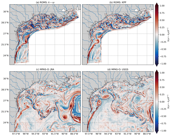
# Review of "Towards high-fidelity simulations of coastal submesoscale baroclinic instabilities with MPAS-O (vE3SM3.0.0) Part II: Realistic experiments" by Schlichting et al.## general remarks:Using a novel global MPAS-O configuration with regional grid refinement, the authors investigate the impact of river runoff on submesoscale dynamics in a realistic estuarine environment and compare the results with those from ROMS. Overall, the manuscript is well written and well structured. The model configurations are described in sufficient detail, and the results are presented and discussed clearly.However, the manuscript lacks a clear motivation and a discussion of the current state of the art. In particular, the authors should provide more context on how river runoff is currently represented in global ocean models, and why this becomes a limitation in high res models and why these improvements are scientifically relevant. For example, the implications for biogeochemical processes, carbon uptake in estuaries, or ecosystem studies could be highlighted. It would also be useful to discuss alternative approaches for improving the representation of estuarine dynamics, such as regional models (e.g., GETM) or global models with coastal grid refinement.Furthermore, the authors should clearly define what they mean by "submesoscale dynamics." (see e.g. McWilliams 2016, Mahadevan 2016 Gula 2021) The manuscript would benefit from a discussion of the horizontal resolution required to adequately resolve submesoscale processes throughout the seasonal cycle, both on the shelf and in the open ocean. In addition, the authors should clarify which submesoscale processes are expected to be resolved by the model and which remain under-resolved (e.g., gravitational, baroclinic, and symmetric instabilities).The authors argue that submesoscale eddies are suppressed during winter, (either due to wind forcing or insufficient model resolution?), and that this affects the estuarine volume transport. However, the figures appear to show more eddy activity during winter than during summer. This apparent contradiction should be resolved and discussed in greater detail.Finally, the manuscript lacks an evaluation against observations, which is important for assessing the realism of the simulated dynamics. While ROMS is used as the reference model, it would strengthen the manuscript if the authors briefly discussed how well ROMS reproduces observations in this region, drawing on previous validation studies where available. For example; do we expect a brackish lense, as seen in MPAS-O, in the estuary or not?Other comments:L26: There are also studies using unstructured-grid models to investigate submesoscale processes, for example, the work by Uchida et al. (2022) (including FESOM) and Epke et al. (2025).L31: Please clarify what is meant by a surface-advected submesoscale eddy field. It would also be helpful to briefly describe the background coastal circulation.L36: Please mention that the growth rate of mixed-layer instabilities scales with mixed layer depth (MLD) and that enhanced submesoscale activity during winter is a well-established result, e.g. see Mahadevan (2016.)L50: Consider mentioning GETM here as an alternative approach for representing rivers and estuaries, and briefly discuss how similar concepts could be incorporated into global ocean models.L56: Please clarify what is meant by coastal processes being "ill-posed." Which specific processes or limitations are being referred to?L57: Please be more specific about the numerical errors and physical processes being discussed. The explanation should be sufficiently self-contained so that readers do not need to consult the cited paper.L60: This paragraph seems out of place. The section should first introduce its objectives before discussing the model setup.L102: Please refer to Fig. 4 here so that readers can directly assess the seasonal variability.L108: It would be useful to briefly explain how temperature is prescribed in this approach.L162: What is the vertical distribution of the river runoff in MPAS-O? Is the runoff applied only at the surface, or is it distributed over multiple vertical levels?L167: Please clarify how river runoff is implemented in MPAS-O. Is the runoff applied to individual coastal grid cells or several? Does it mean there is no spreading of the river runoff in MPAS-O: USGS simulation?L198: Changing the temperature of the run of to (10 m JRA air temperature) is only performed to reduce spurious spikes in the sst? Is this change applicable to other regions (e.g. high latitudes) or is it specific to this estuary?L201: Please clarify this statement. Does the model fail to produce these features only during the final simulation year, or throughout the entire simulation period?L208: Relative vorticity is typically normalized by the Coriolis parameter, yielding the Rossby number. Large Rossby numbers indicate ageostrophic motions and are commonly used as an indicator of submesoscale dynamics. It is therefore unclear what the authors mean by normalized relative vorticity. Since the Rossby number is already nondimensional, the current terminology is potentially misleading. Please clarify the definition and explain whether an additional normalization has been applied.L211: The wording in this paragraph is imprecise, and several terms are used inconsistently. For example, what is meant by a chaotic front - rather unstable fronts, however this needs to be shown... The authors should use more precise terminology throughout this discussion.A more convincing analysis would combine the Rossby number with a snapshot of the lateral buoyancy gradient. The authors could then state, for example: "Large Rossby numbers are found throughout the domain, indicating ageostrophic motions that are commonly associated with submesoscale dynamics. This is consistent with the presence of numerous fronts visible in the lateral buoyancy gradient field (Fig. XX)." However, while the presence of fronts and elevated Rossby numbers is consistent with submesoscale activity, it does not demonstrate the underlying generation mechanism. The manuscript currently infers that these features arise from instabilities, but this is not shown. To support this interpretation, the authors could evaluate additional diagnostics, such as the Richardson number or criteria for mixed-layer/baroclinic instabilities, to demonstrate that the observed structures are indeed generated by baroclinic instability.Finally, based on the figures presented, it is not obvious that submesoscale dynamics are more prevalent on the continental shelf than offshore. This conclusion should either be supported with quantitative diagnostics or stated more cautiously.L213f: An assessment of the relevant horizontal length scales required to resolve mixed-layer baroclinic instabilities is missing. In the open ocean, the characteristic scale is typically given by the mixed-layer deformation radius (see e.g. Dong (2020) et al., Epke (2025) et al.). It is unclear whether this scaling also applies in the coastal and estuarine regions considered here, where stratification and topographic effects may modify the relevant length scales. The authors should provide a clear scale analysis and compare the resulting length scales to the effective horizontal resolution of the model. This is important, as insufficient resolution may lead to a suppression or underrepresentation of submesoscale dynamics. The authors might include this diagnostic in the manuscript to support their conclusions regarding the presence or absence of submesoscale features in different regions and seasons.L224f: The mechanism by which river discharge suppresses mixed-layer instabilities is not clearly explained. Please clarify how freshwater input modifies the stratification and mixed-layer depth, and how this in turn affects instability growth. The phrase interplay between stratification and mixed-layer depth is too vague and should be made more explicit in physical terms.L236: The statement is not consistent with what is shown in Figs. 5. The figures appear to indicate more eddy activity on the shelf during winter than during summer. This discrepancy should be clarified and discussed. In addition, the change in colorbar scaling between panels is not helpful for comparison. For consistency, the Rossby number should be shown using a fixed range (e.g. -1 to 1) across all relevant figures.L256: Again, the terminology should be revised to use Rossby number consistently rather than normalized relative vorticity (see comment on L208).L261: The term realistic eddies is unclear and should be defined more precisely. Also mention that the reference meant here is ROMS.L270: The definition of surface boundary layer depth is not provided. It should be specified whether this corresponds to the mixed layer depth or another diagnostic quantity, and how it is calculated. The same clarification is needed in L272. A comparison of the mixed layer depth with available climatologies would be very helpful to assess realism. In addition, it would be useful to discuss whether the simulated freshwater lens in the estuary is realistic and how it compares to observational estimates.L281: Eddy suppression is not clearly defined. It is unclear whether this refers to suppression of mixed-layer eddies due to insufficient horizontal resolution in MPAS-O, due to atmospheric forcing (e.g. winds), or due to other physical or numerical factors.L283: The main conclusion of this paragraph is not clearly stated. If the authors are suggesting modifications to the KPP scheme in MPAS-O based on ROMS behavior, this recommendation should be made explicit and supported more clearly.L302: It is unclear which model exhibits a larger freshwater volume—MPAS-O or ROMS. The authors suggest that reduced freshwater volume in MPAS-O may be linked to fewer mixed-layer eddies, but this relationship is not demonstrated. This could also be influenced by differences in the vertical mixing parameterization, in particular the KPP scheme. Please clarify.L375: The statement regarding eddy suppression in winter is not consistent with the diagnostics shown earlier. This needs to be reconsidered in light of the Rossby number fields (see related comments above).L385: This interpretation appears incorrect. The figures of Rossby number indicate the opposite trend, namely stronger eddy activity during winter compared to summer. The same concern applies to L404. This discrepancy should be resolved.L419: It would be useful to show instantaneous or spatial fields of surface density gradients, rather than only domain-averaged quantities, to better support the interpretation of the results.Uchida, T. et al. Cloud-based framework for inter-comparing submesoscale-permitting realistic ocean models. Geosci. Model Dev. 15, 5829–5856 (2022).Epke, M., Linardakis, L., Korn, P. & Brüggemann, N. Overturning of mixed layer eddies in a submesoscale resolving simulation of the North Atlantic. J. Phys. Oceanogr. 1–66 (2025) doi:10.1175/JPO-D-25-0015.1.Mahadevan, A. The Impact of Submesoscale Physics on Primary Productivity of Plankton. Ann. Rev. Mar. Sci. 8, 161–184 (2016).Dong, J., Fox-Kemper, B., Zhang, H. & Dong, C. The scale of submesoscale baroclinic instability globally. J. Phys. Oceanogr. 50, 2649–2667 (2020).Gula, J., Taylor, J., Shcherbina, A. & Mahadevan, A. Submesoscale processes and Mix- ing. 1–62 (2021).McWilliams, J. C. Submesoscale currents in the ocean. Proc. R. Soc. A Math. Phys. Eng. Sci. 472, (2016).Citation: https://doi.org/
10.5194/egusphere-2026-1567-RC1 -
AC1: 'Reply on RC1', Dylan Schlichting, 29 Sep 2026
The comment was uploaded in the form of a supplement: https://egusphere.copernicus.org/preprints/2026/egusphere-2026-1567/egusphere-2026-1567-AC1-supplement.pdf
-
AC1: 'Reply on RC1', Dylan Schlichting, 29 Sep 2026
-
RC2: 'Comment on egusphere-2026-1567', Anonymous Referee #2, 27 Jul 2026
Review of "Towards high-fidelity simulations of coastal submesoscale baroclinic
instabilities with MPAS-O (vE3SM3.0.0) Part II: Realistic
experiments" by D. R. Schlichting, K. M. Smith, M. R. Petersen,
R. D. Hetland, K. E. Hinson and D. EngwirdThis manuscript assesses the ability of a global unstructured-grid ocean model with local mesh refinement to reproduce coastal submesoscale dynamics in the northern Gulf of Mexico.
Two MPAS-O configurations are evaluated (MPAS-O: JRA and MPAS-O: USGS), the latter being specifically designed to better represent the Mississippi-Atchafalaya river plumes in the northern Gulf of Mexico. These simulations are compared with two regional ROMS configurations of the Texas-Louisiana shelf, using KPP and k-omega vertical mixing parameterizations.
Following a detailed description of the model configurations and parameterizations, the authors show that both MPAS-O configurations are able to reproduce the vigorous submesoscale variability of the open Gulf of Mexico reasonably well. However, they fail to realistically reproduce the summer submesoscale eddy field over the Texas-Louisiana shelf. As a consequence, excessive freshwater remains trapped on the inner shelf throughout the year, leading to significant salinity biases relative to the ROMS simulations.
Several hypotheses are proposed to explain these discrepancies, including the sensitivity of the vertical mixing parameterization to tuning, the neglect of horizontal momentum associated with river runoff, or biases arising from bathymetric representation and topographic smoothing.
Overall, this study highlights the potential of unstructured-grid models for representing open-ocean submesoscale dynamics, while also identifying shortcomings that remain for accurately simulating shelf submesoscale processes.
General comments
This manuscript is clear, well written, and easy to follow. The figures are of high quality, and the abstract provides an accurate summary of the work. The paper presents a thorough assessment of the strengths and weaknesses of MPAS-O in representing submesoscale dynamics in the northern Gulf of Mexico compared with dedicated regional ROMS simulations.
My main concern is that the discussion of the causes of the MPAS-O biases, particularly the lack of submesoscale eddies over the shelf, remains somewhat limited.
For example, I was surprised to see that MPAS-O uses a first-order Forward Euler scheme for tracer time stepping. Such a low-order scheme is highly diffusive and may substantially damp tracer gradients and associated submesoscale eddy activity. It would therefore be valuable to assess whether numerical diffusion contributes to the weaker shelf variability. One possible approach would be to compare the effective horizontal resolution of MPAS-O and ROMS using kinetic energy spectra at selected locations, following the methodology of Soufflet et al. (2016).
Another important aspect that deserves more discussion is the representation of bathymetry using the z* vertical coordinate. This coordinate system may significantly affect shelf dynamics because current-topography interactions are generally less accurately represented than in terrain-following coordinate systems. A useful sensitivity test, even on a shorter simulation and perhaps with a coarser horizontal mesh, would be to substantially increase the number of z* levels (for example, to around 200) to evaluate the impact of vertical resolution on shelf circulation and submesoscale dynamics.
Similarly, bathymetric smoothing, commonly applied in terrain-following models such as ROMS, may also contribute to some of the differences between the simulations. This aspect deserves additional discussion and, if feasible, dedicated sensitivity experiments.
Overall, I believe this is a valuable contribution, and I recommend publication after minor revisions.
Specific comments
- Throughout the manuscript, a large number of acronyms are introduced (e.g., RYF, SYPD, etc.). Reducing the number of acronyms to only those that are essential would improve readability.
- Table 1: Thank you for providing this clear and detailed summary of the model configurations. I was particularly surprised to see that MPAS-O uses a first-order Forward Euler scheme for tracer time stepping, as this choice may have important implications for the representation of submesoscale dynamics.
- Line 113: "five years on 120 CPU cores" is this correct? Could this instead refer to 120 compute nodes?
- Line 157: I would expect the influence of sea ice on the representation of the Loop Current (LC) to be largely indirect, through large-scale circulation changes (e.g., the MOC), rather than through local processes. This point may be beyond the scope of the present study.
References
Soufflet, Y., P. Marchesiello, F. Lemarie, J. Jouanno, X. Capet, L. Debreu, R. Benshila, On effective resolution in ocean models, Ocean Modelling, 2016, 98, 36-50.
Citation: https://doi.org/10.5194/egusphere-2026-1567-RC2 -
AC2: 'Reply on RC2', Dylan Schlichting, 29 Sep 2026
The comment was uploaded in the form of a supplement: https://egusphere.copernicus.org/preprints/2026/egusphere-2026-1567/egusphere-2026-1567-AC2-supplement.pdf
-
AC2: 'Reply on RC2', Dylan Schlichting, 29 Sep 2026
Peer review completion


Interactive discussion
Status: closed
-
RC1: 'Comment on egusphere-2026-1567', Anonymous Referee #1, 06 Jul 2026
# Review of "Towards high-fidelity simulations of coastal submesoscale baroclinic instabilities with MPAS-O (vE3SM3.0.0) Part II: Realistic experiments" by Schlichting et al.## general remarks:Using a novel global MPAS-O configuration with regional grid refinement, the authors investigate the impact of river runoff on submesoscale dynamics in a realistic estuarine environment and compare the results with those from ROMS. Overall, the manuscript is well written and well structured. The model configurations are described in sufficient detail, and the results are presented and discussed clearly.However, the manuscript lacks a clear motivation and a discussion of the current state of the art. In particular, the authors should provide more context on how river runoff is currently represented in global ocean models, and why this becomes a limitation in high res models and why these improvements are scientifically relevant. For example, the implications for biogeochemical processes, carbon uptake in estuaries, or ecosystem studies could be highlighted. It would also be useful to discuss alternative approaches for improving the representation of estuarine dynamics, such as regional models (e.g., GETM) or global models with coastal grid refinement.Furthermore, the authors should clearly define what they mean by "submesoscale dynamics." (see e.g. McWilliams 2016, Mahadevan 2016 Gula 2021) The manuscript would benefit from a discussion of the horizontal resolution required to adequately resolve submesoscale processes throughout the seasonal cycle, both on the shelf and in the open ocean. In addition, the authors should clarify which submesoscale processes are expected to be resolved by the model and which remain under-resolved (e.g., gravitational, baroclinic, and symmetric instabilities).The authors argue that submesoscale eddies are suppressed during winter, (either due to wind forcing or insufficient model resolution?), and that this affects the estuarine volume transport. However, the figures appear to show more eddy activity during winter than during summer. This apparent contradiction should be resolved and discussed in greater detail.Finally, the manuscript lacks an evaluation against observations, which is important for assessing the realism of the simulated dynamics. While ROMS is used as the reference model, it would strengthen the manuscript if the authors briefly discussed how well ROMS reproduces observations in this region, drawing on previous validation studies where available. For example; do we expect a brackish lense, as seen in MPAS-O, in the estuary or not?Other comments:L26: There are also studies using unstructured-grid models to investigate submesoscale processes, for example, the work by Uchida et al. (2022) (including FESOM) and Epke et al. (2025).L31: Please clarify what is meant by a surface-advected submesoscale eddy field. It would also be helpful to briefly describe the background coastal circulation.L36: Please mention that the growth rate of mixed-layer instabilities scales with mixed layer depth (MLD) and that enhanced submesoscale activity during winter is a well-established result, e.g. see Mahadevan (2016.)L50: Consider mentioning GETM here as an alternative approach for representing rivers and estuaries, and briefly discuss how similar concepts could be incorporated into global ocean models.L56: Please clarify what is meant by coastal processes being "ill-posed." Which specific processes or limitations are being referred to?L57: Please be more specific about the numerical errors and physical processes being discussed. The explanation should be sufficiently self-contained so that readers do not need to consult the cited paper.L60: This paragraph seems out of place. The section should first introduce its objectives before discussing the model setup.L102: Please refer to Fig. 4 here so that readers can directly assess the seasonal variability.L108: It would be useful to briefly explain how temperature is prescribed in this approach.L162: What is the vertical distribution of the river runoff in MPAS-O? Is the runoff applied only at the surface, or is it distributed over multiple vertical levels?L167: Please clarify how river runoff is implemented in MPAS-O. Is the runoff applied to individual coastal grid cells or several? Does it mean there is no spreading of the river runoff in MPAS-O: USGS simulation?L198: Changing the temperature of the run of to (10 m JRA air temperature) is only performed to reduce spurious spikes in the sst? Is this change applicable to other regions (e.g. high latitudes) or is it specific to this estuary?L201: Please clarify this statement. Does the model fail to produce these features only during the final simulation year, or throughout the entire simulation period?L208: Relative vorticity is typically normalized by the Coriolis parameter, yielding the Rossby number. Large Rossby numbers indicate ageostrophic motions and are commonly used as an indicator of submesoscale dynamics. It is therefore unclear what the authors mean by normalized relative vorticity. Since the Rossby number is already nondimensional, the current terminology is potentially misleading. Please clarify the definition and explain whether an additional normalization has been applied.L211: The wording in this paragraph is imprecise, and several terms are used inconsistently. For example, what is meant by a chaotic front - rather unstable fronts, however this needs to be shown... The authors should use more precise terminology throughout this discussion.A more convincing analysis would combine the Rossby number with a snapshot of the lateral buoyancy gradient. The authors could then state, for example: "Large Rossby numbers are found throughout the domain, indicating ageostrophic motions that are commonly associated with submesoscale dynamics. This is consistent with the presence of numerous fronts visible in the lateral buoyancy gradient field (Fig. XX)." However, while the presence of fronts and elevated Rossby numbers is consistent with submesoscale activity, it does not demonstrate the underlying generation mechanism. The manuscript currently infers that these features arise from instabilities, but this is not shown. To support this interpretation, the authors could evaluate additional diagnostics, such as the Richardson number or criteria for mixed-layer/baroclinic instabilities, to demonstrate that the observed structures are indeed generated by baroclinic instability.Finally, based on the figures presented, it is not obvious that submesoscale dynamics are more prevalent on the continental shelf than offshore. This conclusion should either be supported with quantitative diagnostics or stated more cautiously.L213f: An assessment of the relevant horizontal length scales required to resolve mixed-layer baroclinic instabilities is missing. In the open ocean, the characteristic scale is typically given by the mixed-layer deformation radius (see e.g. Dong (2020) et al., Epke (2025) et al.). It is unclear whether this scaling also applies in the coastal and estuarine regions considered here, where stratification and topographic effects may modify the relevant length scales. The authors should provide a clear scale analysis and compare the resulting length scales to the effective horizontal resolution of the model. This is important, as insufficient resolution may lead to a suppression or underrepresentation of submesoscale dynamics. The authors might include this diagnostic in the manuscript to support their conclusions regarding the presence or absence of submesoscale features in different regions and seasons.L224f: The mechanism by which river discharge suppresses mixed-layer instabilities is not clearly explained. Please clarify how freshwater input modifies the stratification and mixed-layer depth, and how this in turn affects instability growth. The phrase interplay between stratification and mixed-layer depth is too vague and should be made more explicit in physical terms.L236: The statement is not consistent with what is shown in Figs. 5. The figures appear to indicate more eddy activity on the shelf during winter than during summer. This discrepancy should be clarified and discussed. In addition, the change in colorbar scaling between panels is not helpful for comparison. For consistency, the Rossby number should be shown using a fixed range (e.g. -1 to 1) across all relevant figures.L256: Again, the terminology should be revised to use Rossby number consistently rather than normalized relative vorticity (see comment on L208).L261: The term realistic eddies is unclear and should be defined more precisely. Also mention that the reference meant here is ROMS.L270: The definition of surface boundary layer depth is not provided. It should be specified whether this corresponds to the mixed layer depth or another diagnostic quantity, and how it is calculated. The same clarification is needed in L272. A comparison of the mixed layer depth with available climatologies would be very helpful to assess realism. In addition, it would be useful to discuss whether the simulated freshwater lens in the estuary is realistic and how it compares to observational estimates.L281: Eddy suppression is not clearly defined. It is unclear whether this refers to suppression of mixed-layer eddies due to insufficient horizontal resolution in MPAS-O, due to atmospheric forcing (e.g. winds), or due to other physical or numerical factors.L283: The main conclusion of this paragraph is not clearly stated. If the authors are suggesting modifications to the KPP scheme in MPAS-O based on ROMS behavior, this recommendation should be made explicit and supported more clearly.L302: It is unclear which model exhibits a larger freshwater volume—MPAS-O or ROMS. The authors suggest that reduced freshwater volume in MPAS-O may be linked to fewer mixed-layer eddies, but this relationship is not demonstrated. This could also be influenced by differences in the vertical mixing parameterization, in particular the KPP scheme. Please clarify.L375: The statement regarding eddy suppression in winter is not consistent with the diagnostics shown earlier. This needs to be reconsidered in light of the Rossby number fields (see related comments above).L385: This interpretation appears incorrect. The figures of Rossby number indicate the opposite trend, namely stronger eddy activity during winter compared to summer. The same concern applies to L404. This discrepancy should be resolved.L419: It would be useful to show instantaneous or spatial fields of surface density gradients, rather than only domain-averaged quantities, to better support the interpretation of the results.Uchida, T. et al. Cloud-based framework for inter-comparing submesoscale-permitting realistic ocean models. Geosci. Model Dev. 15, 5829–5856 (2022).Epke, M., Linardakis, L., Korn, P. & Brüggemann, N. Overturning of mixed layer eddies in a submesoscale resolving simulation of the North Atlantic. J. Phys. Oceanogr. 1–66 (2025) doi:10.1175/JPO-D-25-0015.1.Mahadevan, A. The Impact of Submesoscale Physics on Primary Productivity of Plankton. Ann. Rev. Mar. Sci. 8, 161–184 (2016).Dong, J., Fox-Kemper, B., Zhang, H. & Dong, C. The scale of submesoscale baroclinic instability globally. J. Phys. Oceanogr. 50, 2649–2667 (2020).Gula, J., Taylor, J., Shcherbina, A. & Mahadevan, A. Submesoscale processes and Mix- ing. 1–62 (2021).McWilliams, J. C. Submesoscale currents in the ocean. Proc. R. Soc. A Math. Phys. Eng. Sci. 472, (2016).Citation: https://doi.org/
10.5194/egusphere-2026-1567-RC1 -
AC1: 'Reply on RC1', Dylan Schlichting, 29 Sep 2026
The comment was uploaded in the form of a supplement: https://egusphere.copernicus.org/preprints/2026/egusphere-2026-1567/egusphere-2026-1567-AC1-supplement.pdf
-
AC1: 'Reply on RC1', Dylan Schlichting, 29 Sep 2026
-
RC2: 'Comment on egusphere-2026-1567', Anonymous Referee #2, 27 Jul 2026
Review of "Towards high-fidelity simulations of coastal submesoscale baroclinic
instabilities with MPAS-O (vE3SM3.0.0) Part II: Realistic
experiments" by D. R. Schlichting, K. M. Smith, M. R. Petersen,
R. D. Hetland, K. E. Hinson and D. EngwirdThis manuscript assesses the ability of a global unstructured-grid ocean model with local mesh refinement to reproduce coastal submesoscale dynamics in the northern Gulf of Mexico.
Two MPAS-O configurations are evaluated (MPAS-O: JRA and MPAS-O: USGS), the latter being specifically designed to better represent the Mississippi-Atchafalaya river plumes in the northern Gulf of Mexico. These simulations are compared with two regional ROMS configurations of the Texas-Louisiana shelf, using KPP and k-omega vertical mixing parameterizations.
Following a detailed description of the model configurations and parameterizations, the authors show that both MPAS-O configurations are able to reproduce the vigorous submesoscale variability of the open Gulf of Mexico reasonably well. However, they fail to realistically reproduce the summer submesoscale eddy field over the Texas-Louisiana shelf. As a consequence, excessive freshwater remains trapped on the inner shelf throughout the year, leading to significant salinity biases relative to the ROMS simulations.
Several hypotheses are proposed to explain these discrepancies, including the sensitivity of the vertical mixing parameterization to tuning, the neglect of horizontal momentum associated with river runoff, or biases arising from bathymetric representation and topographic smoothing.
Overall, this study highlights the potential of unstructured-grid models for representing open-ocean submesoscale dynamics, while also identifying shortcomings that remain for accurately simulating shelf submesoscale processes.
General comments
This manuscript is clear, well written, and easy to follow. The figures are of high quality, and the abstract provides an accurate summary of the work. The paper presents a thorough assessment of the strengths and weaknesses of MPAS-O in representing submesoscale dynamics in the northern Gulf of Mexico compared with dedicated regional ROMS simulations.
My main concern is that the discussion of the causes of the MPAS-O biases, particularly the lack of submesoscale eddies over the shelf, remains somewhat limited.
For example, I was surprised to see that MPAS-O uses a first-order Forward Euler scheme for tracer time stepping. Such a low-order scheme is highly diffusive and may substantially damp tracer gradients and associated submesoscale eddy activity. It would therefore be valuable to assess whether numerical diffusion contributes to the weaker shelf variability. One possible approach would be to compare the effective horizontal resolution of MPAS-O and ROMS using kinetic energy spectra at selected locations, following the methodology of Soufflet et al. (2016).
Another important aspect that deserves more discussion is the representation of bathymetry using the z* vertical coordinate. This coordinate system may significantly affect shelf dynamics because current-topography interactions are generally less accurately represented than in terrain-following coordinate systems. A useful sensitivity test, even on a shorter simulation and perhaps with a coarser horizontal mesh, would be to substantially increase the number of z* levels (for example, to around 200) to evaluate the impact of vertical resolution on shelf circulation and submesoscale dynamics.
Similarly, bathymetric smoothing, commonly applied in terrain-following models such as ROMS, may also contribute to some of the differences between the simulations. This aspect deserves additional discussion and, if feasible, dedicated sensitivity experiments.
Overall, I believe this is a valuable contribution, and I recommend publication after minor revisions.
Specific comments
- Throughout the manuscript, a large number of acronyms are introduced (e.g., RYF, SYPD, etc.). Reducing the number of acronyms to only those that are essential would improve readability.
- Table 1: Thank you for providing this clear and detailed summary of the model configurations. I was particularly surprised to see that MPAS-O uses a first-order Forward Euler scheme for tracer time stepping, as this choice may have important implications for the representation of submesoscale dynamics.
- Line 113: "five years on 120 CPU cores" is this correct? Could this instead refer to 120 compute nodes?
- Line 157: I would expect the influence of sea ice on the representation of the Loop Current (LC) to be largely indirect, through large-scale circulation changes (e.g., the MOC), rather than through local processes. This point may be beyond the scope of the present study.
References
Soufflet, Y., P. Marchesiello, F. Lemarie, J. Jouanno, X. Capet, L. Debreu, R. Benshila, On effective resolution in ocean models, Ocean Modelling, 2016, 98, 36-50.
Citation: https://doi.org/10.5194/egusphere-2026-1567-RC2 -
AC2: 'Reply on RC2', Dylan Schlichting, 29 Sep 2026
The comment was uploaded in the form of a supplement: https://egusphere.copernicus.org/preprints/2026/egusphere-2026-1567/egusphere-2026-1567-AC2-supplement.pdf
-
AC2: 'Reply on RC2', Dylan Schlichting, 29 Sep 2026
Peer review completion
Journal article(s) based on this preprint
Data sets
Towards high-fidelity simulations of coastal submesoscale baroclinic instabilities with MPAS-O Part II: Realistic experiments Dylan Schlichting et al. https://doi.org/10.5281/zenodo.17903087
Viewed
| HTML | XML | Total | BibTeX | EndNote | |
|---|---|---|---|---|---|
| 299 | 171 | 45 | 515 | 31 | 29 |
- HTML: 299
- PDF: 171
- XML: 45
- Total: 515
- BibTeX: 31
- EndNote: 29
Viewed (geographical distribution)
| Country | # | Views | % |
|---|
| Total: | 0 |
| HTML: | 0 |
| PDF: | 0 |
| XML: | 0 |
- 1

Katherine Smith
Mark Petersen
Robert Hetland
Kyle Hinson
Darren Engwirda
The requested preprint has a corresponding peer-reviewed final revised paper. You are encouraged to refer to the final revised version.
- Preprint
(30675 KB) - Metadata XML