
the Creative Commons Attribution 4.0 License.
the Creative Commons Attribution 4.0 License.
 | 07 Apr 2026
Assessing Financial Risk to Property Portfolios from Physical Rainfall Extremes
Abstract. Physical climate risk from extreme rainfall is often poorly understood by financial investors, potentially extending to pension funds that manage assets of substantial societal importance. There is a growing need for investors to better understand these risks to ensure financial resilience in a changing climate. We present a transparent framework to estimate current and near-future financial risk from flood damage using rainfall hazard information from regional climate projections, river flood maps, and depth-damage functions. Synthetic portfolios are constructed from non-residential built-up surface data and country-specific property values, enabling calculation of Expected Annual Damage. Results show that this physical climate risk is already substantial and projected to rise consistently across Europe, with some regions experiencing particularly large increases. Portfolio composition strongly influences risk, with asset location and value at-risk inducing greater variability than climate model uncertainty. We also demonstrate how adaptation could significantly reduce EAD and deliver a strong financial return within a short time frame, reinforcing its role as a cost-effective strategy for managing climate-related risks. This approach offers a pragmatic and transparent method for quantifying an element of financial risk from extreme rainfall using openly available datasets. Our approach is intended primarily for demonstration and awareness purposes, given its limitations such as the simplified modelling of rainfall–flood relationships and the omission of potential future changes to floodplains. Nonetheless, the findings highlight the urgent need for financial actors, such as asset managers, to integrate physical climate risk into decision-making to safeguard long-term financial resilience.
-
Notice on discussion status
The requested preprint has a corresponding peer-reviewed final revised paper. You are encouraged to refer to the final revised version.
-
Preprint
(63602 KB)
-
Supplement
(1401 KB)
-
The requested preprint has a corresponding peer-reviewed final revised paper. You are encouraged to refer to the final revised version.
- Preprint
(63602 KB) - Metadata XML
-
Supplement
(1401 KB) - BibTeX
- EndNote
- Final revised paper


Journal article(s) based on this preprint
Interactive discussion
Status: closed
-
RC1: 'Comment on egusphere-2026-1142', Anonymous Referee #1, 04 May 2026
-
AC1: 'Reply on RC1', Laura Dawkins, 01 Jul 2026
We are grateful to the reviewer for their thoughtful and constructive feedback, and for the time taken to engage so carefully with the manuscript. We have implemented a number of changes in response to these suggestions, which we feel have significantly improved the paper.
Please see the attached document for a detailed reply to all of the reviewer comments. We have included both RC1 and RC2 in the document as we refer to both in places.
-
AC1: 'Reply on RC1', Laura Dawkins, 01 Jul 2026
-
RC2: 'Comment on egusphere-2026-1142', Anonymous Referee #2, 11 May 2026
The paper addresses a highly relevant topic—financial risk associated with extreme rainfall and flooding—and proposes a transparent framework based on open data. The proposal is useful as a demonstrative and educational framework. However, there are substantial methodological limitations, some acknowledged by the authors, that reduce the quantitative robustness of the conclusions.
Below are some points that, in my opinion, should be clarified and explored in more depth in the paper:
- Discuss the inconsistency between the different spatial resolutions used (12 km for rainfall versus 100 m for flooding and financial assets);
- Lines 320-325: Explain under what physical conditions the rainfall → flood depth approximation can be considered valid.
- The entire methodology relies on statistical mapping and does not present explicit observational validation; especially Section 2.2.3 and Section 5. Is it possible to include independent validation using observed flood data, actual economic losses, or official risk maps?
- Section 2.2.3: Justify the implicit assumption of stationarity of the rainfall-flood relationship under future climate change.
- Figure 8: Discuss the limitations associated with the use of national average property values, ignoring intra-urban and regional heterogeneity.
- Lines 599-605: Better justify the simplified relationship between precipitation extremes and flood depth, considering that the method ignores fundamental hydrological processes.
- Lines 620-645: Better justify the exclusive use of a single climate scenario and discuss differences under intermediate scenarios.
- Is it possible to present a sensitivity or stability analysis of the extrapolation performed by the monotonic spline?
- Discuss in more depth the impacts of the absence of bias correction on the final monetary results.
- Lines 628-635: Explain how random synthetic portfolios adequately represent real financial portfolios.
- Figure 13: Discuss the limitations of the simplified modeling of adaptation and flood protection measures.
- Caution: Moderate the language of the conclusions, as the paper itself acknowledges that the framework is exploratory and demonstrative in nature.
Citation: https://doi.org/10.5194/egusphere-2026-1142-RC2 -
AC2: 'Reply on RC2', Laura Dawkins, 01 Jul 2026
We are grateful to the reviewer for their thoughtful and constructive feedback, and for the time taken to engage so carefully with the manuscript. We have implemented a number of changes in response to these suggestions, which we feel have significantly improved the paper.
Please see the attached document for a detailed reply to all of the reviewer comments. We have included both RC1 and RC2 in the document as we refer to both in places.
Peer review completion


Interactive discussion
Status: closed
-
RC1: 'Comment on egusphere-2026-1142', Anonymous Referee #1, 04 May 2026
Dawkins et al have presented a portfolio level assessment of expected damages from rainfall induced floods for non-residential built area across Europe. Given the dearth of broadly applicable spatial data and lack of international hydrological modeling, this is a well written and commendable effort to provide a data driven approach to estimating portfolio risk, especially for insurance and pension plan providers.
Based on my review, I noted a few major issues like the mapping from rainfall to flood hazard, inaccuracies such as calculation of AEP, and unclear figures. I also noted a few minor corrections. Hopefully the authors and the editor would find these comments insightful and beneficial for improving the manuscript for future readers.
- One of the primary limitations of this study is the mapping step from rainfall hazard to flood hazard. No validation has been provided for the approach, and this step severely limits the applicability of this study. While the authors have pointed out in the limitations section that their analysis is illustrative, it would be good to emphasize this limitation both in the Limitations section and throughout the manuscript.
- Line 324: I am not convinced that there would be 1:1 mapping between the X-year return period rainfall and X-year return period flood. Surely, multiple rainfall events could cause the same flooding, and in its most accurate form, each flood hazard curve would be a weighted integration of the rainfall’s entire spatio-temporal probability distribution. Can the authors provide justification for this simplification?
- Line 366: From figure 6, it appears that Gothenburg and Edinburgh were both used for fitting the splines, so it creates a circular logic to both fit the data to the CEMS data points and to state that the fitted curves align well with the CEMS data points.
- Line 231: Why does only scale vary spatially, and not shape?
- Line 232: Is the spatial variation of scale from this method parametric or non-parametric? If parametric, it will be helpful for the readers to include its functional form. If non-parametric, can you specify the spatial grid spacing, and how the 12 km dataset is mapped on to this spatial grid?
- Line 249: It does not appear that there are any temporal parameters in the fitted distribution. Is the assumption that the distribution parameters are constant over the entirety of each time period? Is that a fair assumption, especially given the authors’ statement in the Introduction about 25% of flood losses observed within the most recent 3 years of the last 44?
- Paragraph 291: Can the authors include some comments on the QQplots at higher quantiles? The variation is typically largest at the highest quantiles, which is exactly the region that is being intended to be modeled by the EV-GAM. Did the authors notice a systematic under- or over-estimation in this region? What is causing this misfit, and how would adding covariates help reduce this misfit?
- Paragraph 291: Did the authors explore other probability distributions to model the rainfall data? Since the UKCP18 data includes forecasts, what distributions does that data use, and how does it differ from the authors’ choice?
- Line 306: The number of simulated data points seem to be too low for modeling more than ~10 years return period. For example, 500 years would have >180k days, and assuming 10 data points for achieving statistical significance, 1.8M data points would be required. Is there something I am missing from the description of the simulation approach, e.g., that only extreme rainfall events are simulated in which case how is their probability accounted for in the hazard curve generation?
- Line 303: Given the above comment, it is not completely clear to me why the authors needed to first fit the UKCP18 data to EV-GAM, and then simulate daily rainfall, instead of using the daily rainfall data directly? Over the 30 year time periods, there are already ~11k data points. Are the hazard values obtained from the simulated approach significantly different than if the authors had used the data directly?
- Line 461: Since the vulnerability function is a CDF, can the authors comment on their choice to use a spline fit instead of fitting a probability distribution, like lognormal?
- Line 471: It would help the readers better understand the methodology if the authors included the integration equation to illustrate how the hazard curve is combined with the vulnerability function? Additionally, closed form integration is generally not possible so can the authors also include their discretization step size?
- Figure 9 and line 484: While it is a reasonably good assumption for quick calculations, the authors have incorrectly stated that AEP is the inverse of the return period (otherwise for a 6-month return period, the annual exceedance probability will be 2, which is impossible). Please include the correct conversion based on the Poisson distribution to convert return periods to AEP.
- Paragraph 496: It will be helpful if the authors can present actual loss damages from any recent flooding events at one of the presented cities, especially if that event’s return period is quantified. This would help the authors validate their EAD estimates, and help readers anchor this study’s EAD calculations, otherwise it is difficult to verify their order of magnitude.
- Line 508: Why are there ensemble members for the historical time period? Wouldn’t the historical data be static and known, and ensembles only be present for future forecasted scenarios?
- Line 537: It would be interesting to see the variability in estimates for simulated portfolios with the same flood risk sampling, e.g., 1000 portfolios with 20% flood-risk regions, and 1000 portfolios with 80% flood-risk regions. This would test the hypothesis whether the percentage of built area in flood risk regions is by itself a good proxy for EAD.
- Figure 12: It is not clear why the authors chose the particular distribution of the portfolio samples in panel b. In fact the variability in panel b appears less than that of panel a, which appears counter-intuitive. Separate plots with 1000 samples at the same flood risk percentage might be more helpful to compare the effect of flood risk area. A plot showing the flood risk area percent on x-axis with EAD distribution on y-axis would also be informative.
- Paragraph 586: In order to illustrate the recoupment of costs, a discount factor should be added to the EAD.
- Line 48: The authors highlighted variability in vendor estimates for flood risk. However, their manuscript does not address this limitation, nor does it provide a consistent framework that can be used to reduce this variability, especially given their rainfall to flood hazard mapping step. I would encourage the authors to highlight this limitation.
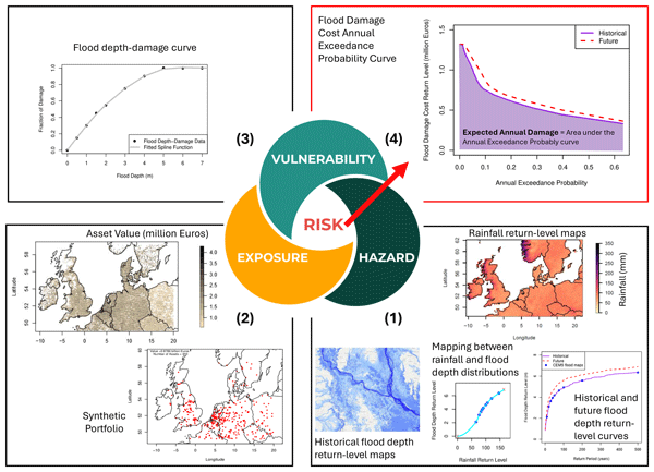
- Figure 1: While the sub-figures represent the various components of the methodology, it is difficult to interpret their flow, as mentioned in paragraph 105. A flowchart or similar step-by-step schematic will make it easier to understand how the figure represents the calculation flow.
- Figure 7: It would be helpful to include the return levels for all 12 ensemble members in the figure, in order to better understand their variability within the main manuscript.
- Figure 8b: Since the value is constant per country, it will be better represented by a table, than a gridded map which gives the impression of more spatial variability.
- Figure 10: Due to the narrow dispersion, the panel (a) is difficult to read. Suggest removing or lightening the horizontal grid, and perhaps splitting the y-axis as Odense is primarily responsible for the extended y-scale. A log y-axis would be another option, given the losses in millions €.
- Figure 10: Can a statement be added in the caption describing the boxplot: whether the boxes represent 25-75 interquantiles, whiskers, etc.?
- Figure 10: Panel (b) map and the histogram are difficult to read, and the differentiation of colors is not apparent.
- Figure 12: Due to significant overlap in the dots, the overlaid ensembles are not informative. I would suggest changing the figure to make it clearer, e.g., showing the mean and standard deviation from the ensembles.
- Figure 12: Why do some sampled portfolios have 0 EAD in panel b?
- Figure 12: The numbering on the ensemble members seem to indicate that there are more than 12 ensemble members(15?). Can the authors add a statement if they selected a subset of ensembles and their selection criteria?
- Figure 13: At AEP = 1, the EAD must be zero as only 0 damage can occur with certainty. The figure does not represent this.
- Figure 13: Can the authors clarify the axes of panel (a). The x-axis seems to represent the Flood hazard AEP, and the y-axis would be the *Expected* flood damage cost. The y-axis scale is in € so it does not seem to represent the “return level”.
- Line 45: What are transition risk tools?
- Line 91: What does “idealised” refer to?
- Line 118: Nit: *Plausible* hazard scenarios is a more representative terminology, but “possible” is also acceptable.
- Line 118: …probabilities *of occurrence*.
- Line 120: Can the authors add references to some existing hazard products, perhaps in the Introduction section, to illustrate that the authors researched for available event sets among widely available hazard products, bolstering their statement that no such event sets exist? This would also support their next paragraph since hazard products at different return levels are available.
- Line 126: Similar to above comment, Figure 1 does not adequately illustrate how the probability distributions will be combined.
- Line 128: Can the authors add a citation for the identified dataset on its first mention?
- Line 272: Figure 3c -> Figure 3d
- Figure 6: Regarding the two additional points, what is the associated y-axis point corresponding to the highest rainfall x-point?
- Line 351: Can the authors elaborate on “several modelling caveats”?
- Line 352: Can the authors provide supporting evidence for the relationships being informative, and an associated citation for their next statement?
- Line 359: Can the authors mark the 60-year return period values on panels a and c?
- Line 368: Can the authors qualify the return-period, e.g., return-level estimates for ≥ 100 years…?
- Line 369: It is unclear to me from the figure why the estimates are notably high if they align with the CEMS flood map values, which are also ≥5m for ~100-yr return periods.
- Line 497: Would it be possible to include the total non-residential property value of the representative 100m cells in Table 1?
- Paragraph 524: Can the differences between the portfolios be described in this paragraph instead of two paragraphs later? This would help readers anchor the differences in EAD.
- Line 526: It would be better to highlight the differences in the spatial distribution rather than the apparent similarity to help readers focus on the relevant differences, e.g., Portfolio 2 appears to have a higher concentration of built area along the coasts.
- Line 536: How is risk of flooding determined: Is it based on flooding depth exceeding some value for a certain X-year hazard?
- Line 541: It is unclear how to compare the variability of the ensemble members and that of EAD.
- Line 554: It is not clear how to conclude from Figure 12b that portfolios with a higher flood risk area have higher EAD. Similarly for the following statement.
- Line 573: Does the conversion from 10-year flood to 6-yr flood apply to all ensemble members?
- Line 587: Can the authors add a citation or justification for their assumed adaptation cost?
Citation: https://doi.org/10.5194/egusphere-2026-1142-RC1 -
AC1: 'Reply on RC1', Laura Dawkins, 01 Jul 2026
We are grateful to the reviewer for their thoughtful and constructive feedback, and for the time taken to engage so carefully with the manuscript. We have implemented a number of changes in response to these suggestions, which we feel have significantly improved the paper.
Please see the attached document for a detailed reply to all of the reviewer comments. We have included both RC1 and RC2 in the document as we refer to both in places.
-
RC2: 'Comment on egusphere-2026-1142', Anonymous Referee #2, 11 May 2026
The paper addresses a highly relevant topic—financial risk associated with extreme rainfall and flooding—and proposes a transparent framework based on open data. The proposal is useful as a demonstrative and educational framework. However, there are substantial methodological limitations, some acknowledged by the authors, that reduce the quantitative robustness of the conclusions.
Below are some points that, in my opinion, should be clarified and explored in more depth in the paper:
- Discuss the inconsistency between the different spatial resolutions used (12 km for rainfall versus 100 m for flooding and financial assets);
- Lines 320-325: Explain under what physical conditions the rainfall → flood depth approximation can be considered valid.
- The entire methodology relies on statistical mapping and does not present explicit observational validation; especially Section 2.2.3 and Section 5. Is it possible to include independent validation using observed flood data, actual economic losses, or official risk maps?
- Section 2.2.3: Justify the implicit assumption of stationarity of the rainfall-flood relationship under future climate change.
- Figure 8: Discuss the limitations associated with the use of national average property values, ignoring intra-urban and regional heterogeneity.
- Lines 599-605: Better justify the simplified relationship between precipitation extremes and flood depth, considering that the method ignores fundamental hydrological processes.
- Lines 620-645: Better justify the exclusive use of a single climate scenario and discuss differences under intermediate scenarios.
- Is it possible to present a sensitivity or stability analysis of the extrapolation performed by the monotonic spline?
- Discuss in more depth the impacts of the absence of bias correction on the final monetary results.
- Lines 628-635: Explain how random synthetic portfolios adequately represent real financial portfolios.
- Figure 13: Discuss the limitations of the simplified modeling of adaptation and flood protection measures.
- Caution: Moderate the language of the conclusions, as the paper itself acknowledges that the framework is exploratory and demonstrative in nature.
Citation: https://doi.org/10.5194/egusphere-2026-1142-RC2 -
AC2: 'Reply on RC2', Laura Dawkins, 01 Jul 2026
We are grateful to the reviewer for their thoughtful and constructive feedback, and for the time taken to engage so carefully with the manuscript. We have implemented a number of changes in response to these suggestions, which we feel have significantly improved the paper.
Please see the attached document for a detailed reply to all of the reviewer comments. We have included both RC1 and RC2 in the document as we refer to both in places.
Peer review completion
Journal article(s) based on this preprint
Viewed
| HTML | XML | Total | Supplement | BibTeX | EndNote | |
|---|---|---|---|---|---|---|
| 418 | 202 | 42 | 662 | 71 | 30 | 27 |
- HTML: 418
- PDF: 202
- XML: 42
- Total: 662
- Supplement: 71
- BibTeX: 30
- EndNote: 27
Viewed (geographical distribution)
| Country | # | Views | % |
|---|
| Total: | 0 |
| HTML: | 0 |
| PDF: | 0 |
| XML: | 0 |
- 1
Laura C. Dawkins

Freya K. Garry
Dan J. Bernie
Jason A. Lowe
Theodoros Economou
The requested preprint has a corresponding peer-reviewed final revised paper. You are encouraged to refer to the final revised version.
- Preprint
(63602 KB) - Metadata XML
-
Supplement
(1401 KB) - BibTeX
- EndNote
- Final revised paper
Dawkins et al have presented a portfolio level assessment of expected damages from rainfall induced floods for non-residential built area across Europe. Given the dearth of broadly applicable spatial data and lack of international hydrological modeling, this is a well written and commendable effort to provide a data driven approach to estimating portfolio risk, especially for insurance and pension plan providers.
Based on my review, I noted a few major issues like the mapping from rainfall to flood hazard, inaccuracies such as calculation of AEP, and unclear figures. I also noted a few minor corrections. Hopefully the authors and the editor would find these comments insightful and beneficial for improving the manuscript for future readers.