
the Creative Commons Attribution 4.0 License.
the Creative Commons Attribution 4.0 License.
 | 24 Mar 2026
Improving aerosol-radiation interaction feedback in AIRWISE operational system
Abstract. Accurate representation of aerosol optical properties remains a key uncertainty in aerosol–radiation interactions in numerical weather prediction models, especially over highly polluted megacities. Operational systems use globally prescribed complex refractive indices (RIs) that inadequately represent regional aerosol composition, inducing biases in surface shortwave radiation (SWDOWN) and boundary layer evolution. In this study, region-specific RIs of aerosols over Delhi are implemented within the Air Quality Warning and Integrated Decision Support System for Emissions (AIRWISE) to quantify their radiative and meteorological impacts during the October 2023–January 2024 season. Sensitivity experiments with RIs of different chemical species indicate reduction in SWDOWN by up to ~80 W m-2 (diurnally ~43 W m-2) during a severe post-monsoon episode. This radiative perturbation decreases surface temperature (~0.2 °C), near-surface wind speed (~0.4 m s-1), and boundary layer height (~200 m), while increasing daytime humidity (3–4 %). Comparable sensitivity is observed during an extreme winter episode under stagnant, humid conditions favorable for haze persistence. Seasonally, monthly mean SWDOWN decreases by 25–37 W m-2 relative to the control simulation, accounting for ~¼ to ⅓ of total aerosol-induced reduction. Evaluation against surface radiation measurements from Winter Fog Experiment (WiFEX 2023–24) at Indira Gandhi International Airport, Delhi shows substantial bias reduction in December 2023 (62 %) and January 2024 (35 %). The revised radiative forcing systematically modifies near-surface thermodynamics and increases PM2.5 concentrations, thereby altering pollution–meteorology feedback in highly polluted urban environments.
-
Notice on discussion status
The requested preprint has a corresponding peer-reviewed final revised paper. You are encouraged to refer to the final revised version.
-
Preprint
(1502 KB)
-
Supplement
(647 KB)
-
The requested preprint has a corresponding peer-reviewed final revised paper. You are encouraged to refer to the final revised version.
- Preprint
(1502 KB) - Metadata XML
-
Supplement
(647 KB) - BibTeX
- EndNote
- Final revised paper


Journal article(s) based on this preprint
Interactive discussion
Status: closed
-
RC1: 'Comment on egusphere-2026-1100', Anonymous Referee #1, 12 May 2026
- AC1: 'Reply on RC1', Sumit Kumar, 09 Jul 2026
-
RC2: 'Comment on egusphere-2026-1100', Anonymous Referee #2, 13 May 2026
The manuscript by Kumar et al. involves implementation of improved optical properties in regional model simulations with WRF-Chem, and quantification of the subsequent influence on biases in surface shortwave radiation and other variables. By using region-specific refractive indices instead of default values, they find reduced shortwave radiation at the surface and reduced biases compared to observations. The study is fairly well-written, and highlights the importance of using region-specific optical properties, but I have several comments as outlined below.
Main comments
Generalizability: The study is done for a few months over a small region in North-India, mainly using observations from only one station in Delhi. In addition, the WRF-Chem simulations use GOCART, which is a fairly simple bulk aerosol scheme (except that dust and sea salt are size resolved). While its numerical efficiency is an advantage over more sophisticated aerosol schemes, GOCART is mostly useful when the focus is on complex gas phase chemistry and not aerosols. In this case the focus is on aerosols, and I therefore wonder about the generalizability of the findings. Can the findings be put in a broader context? Except for the conclusion that it seems to have some importance for near-surface meteorology to use region-specific refractive indices, I am not sure about the usefulness of the results for others. For instance, can you discuss how the use of GOCART vs. a more detailed scheme like MOSAIC could have influenced the results? Are the default refractive indices in the model specific for each aerosol scheme or universal across all WRF-Chem aerosol schemes? I.e., is the necessity for updating the refractive indices specific to GOCART or is it for WRF-Chem in general? Do the authors think the findings would have changed if a more detailed aerosol scheme would have been used, and if so how? I think a discussion of these issues may make the findings more useful for WRF-Chem users that employ more detailed aerosol schemes.
Novelty: Linked to the comment above, I am left wondering how important the updating of refractive indices really is compared to other factors. The discussion section mentions uncertainties due to urban morphology and soil moisture, and touches upon weaknesses of the GOCART scheme and emission inventories. In particular, I think the use of GOCART together with an old emission inventory is a substantial weakness of the present study. The GOCART scheme does not include SOA or nitrate aerosols, which are likely very important contributors to PM2.5 in the region, especially due to large ammonia emissions from agriculture causing formation of nitrate particles. I am of course in favor of updating to more realistic RIs, but the improvement in modelled SWDOWN and meteorological variables seems minor compared to the overall model vs. observation differences. Given also my comment above about the findings being very specific to a certain location and model setup, I am therefore wondering if the study is novel enough for ACP, but I will leave that decision to the Editor.
Length: The results are very specific for WRF-Chem with the GOCART scheme over Delhi. It does not have wider implications, as far as I can tell, other than that those using WRF-Chem should check that the RIs are representative of their region. I would therefore have preferred a shorter paper. One suggestion for shortening is to remove section 3.5 on the monthly-mean picture since those results are largely in line with the prior analysis on the events. Instead, the associated Figure 9 and Table 3 could be moved to the supplementary, and then been discussed, very briefly, in the other subsections. Another thing would be to remove results for domain 1 entirely and only show results for domain 2, unless there is a good reason for keeping the domain 1 results. Results are anyway shown over Delhi, which is included in domain 2.
Specific comments
Title: Do you need both “interaction” and “feedback” in the title, and if so, I think “and” should be added in between?
L15: Should specify whether SWDOWN is incoming/downward or net surface shortwave radiation
L19-20: The ~0.2C decrease in surface temperature only occurs during very few hours in the morning, according to Figure 5, most of the day there is an increase.
L23 “total aerosol-induced reduction”: Do you mean just ARI or is ACI also now included?
L23-25: RMSE is a better measure, and this does not show as good improvement as the mean bias
L28: earth -> Earth
L29: Could also add a reference to a more recent estimate, such as IPCC AR6 Ch. 7:
Forster, P. M., T. Storelvmo, et al. (2021), The Earth’s Energy Budget, Climate Feedbacks, and Climate Sensitivity, in Climate Change 2021: The Physical Science Basis. Contribution of Working Group I to the Sixth Assessment Report of the Intergovernmental Panel on Climate Change, edited by V. Masson-Delmotte, et al., pp. 923–1054, Cambridge University Press, Cambridge, United Kingdom and New York, NY, USA.
L30: I would have added “and climate” after “weather”
L36: Should add a reference after this statement (after “air quality”). For instance one of these:
Sharma, A., C. Venkataraman, K. Muduchuru, V. Singh, A. Kesarkar, S. Ghosh, and S. Dey (2023), Aerosol radiative feedback enhances particulate pollution over India: A process understanding, Atmospheric Environment, 298, 119609, doi: https://doi.org/10.1016/j.atmosenv.2023.119609.
Hodnebrog, Ø., K. Aunan, S. Chowdhury, L. Marelle, G. Myhre, C. W. Stjern, and S. Wang (2025), Strong reduction in near-surface turbulence due to aerosols in South and East Asia, npj Clean Air, 1(1), 9, doi: 10.1038/s44407-025-00009-6.
L53: “mitigating” may be a better word than “regulating”
L62: WRF-Chem has not been introduced/defined yet
L65: I would say also ACI in addition to ARI? Twomey effect, which is mentioned, is ACI.
L78: Should define PM2.5
L78-85: Could mention that dust emissions/concentrations/forcing are very uncertain and differ a lot between different models, e.g.,
Wu, C., Lin, Z., and Liu, X.: The global dust cycle and uncertainty in CMIP5 (Coupled Model Intercomparison Project phase 5) models, Atmos. Chem. Phys., 20, 10401–10425, https://doi.org/10.5194/acp-20-10401-2020, 2020
Haugvaldstad, O. W., Olivié, D., Storelvmo, T., and Schulz, M.: Dust radiative forcing in CMIP6 Earth System models: insights from the AerChemMIP piClim-2xdust experiment, Atmos. Chem. Phys., 25, 13199–13219, https://doi.org/10.5194/acp-25-13199-2025, 2025
L125-126: I find “air quality” a bit superfluous when the following part of the sentence states “regional and urban-scale pollution”
L126-128: Should also mention sulfate and primary organic aerosols
L136 / Figure S1: The caption mentions a star indicating the location of Delhi, but I cannot find a star
L140 “within the first kilometres”: How many kilometres?
L151-153: I assume the convective parameterization is not applied in domain 2? Convection is typically thought to be fairly resolved at grid spacings <4 km (Prein et al., 2015), and it has even proved beneficial to turn off the convection parameterization at grid spacings lower than around 25 km (Vergara-Temprado et al., 2020).
Prein, A. F., W. Langhans, G. Fosser, A. Ferrone, N. Ban, K. Goergen, M. Keller, M. Toelle, O. Gutjahr, F. Feser, E. Brisson, S. Kollet, J. Schmidli, N. P. M. van Lipzig, and R. Leung (2015), A review on regional convection-permitting climate modeling: Demonstrations, prospects, and challenges, Rev. Geophys., 53(2), 323-361, doi: 10.1002/2014rg000475.
Vergara-Temprado, J., N. Ban, D. Panosetti, L. Schlemmer, and C. Schar (2020), Climate Models Permit Convection at Much Coarser Resolutions Than Previously Considered, J. Clim., 33(5), 1915-1933, doi: 10.1175/jcli-d-19-0286.1.
L162-164: Did the simulations use nudging (grid or spectral) towards the ERA5 data?
L166-169: I think this part can be skipped, I believe it is described in the WRF documentation.
L175-176: How was this refining of emissions done? What source of fine-gridded emissions data for Delhi was used?
L182-186: For this study focusing on aerosols, what was the reason for choosing the simple GOCART scheme and not a more detailed aerosol scheme? For instance the sectional aerosol scheme MOSAIC works well with the MOZART chemistry scheme.
L187: I would have split this subsection by renaming “experiment details” to e.g. “refractive indices” or “optical properties”, and added a new subheading “experiments” to line 223.
L191: What kind of aerosols are included in the “other GOCART primary PM2.5” and how are they treated?
L225-228: It would be useful with more informative names of experiments EXP1-EXP5. An alternative could be EXP2 -> RI_dust and similarly for other experiments.
L248-249: Are 2 days enough for the chemistry to spin up, given the coarse resolution of MOZART initial conditions?
L249-250: I did not quite understand the reasoning for only comparing against the outer (10 km) domain and not the inner (2 km) domain. I would think high resolution is important to get a more realistic representation of aerosol concentrations (PM2.5), especially since there may be many local emission sources around Delhi, which is presumably why the authors have chosen to refine the anthropogenic emissions in this region. Is the choice related to lack of observations in the Delhi region? I would think not, because later on it is described that 40 monitoring stations across Delhi are used. On a related note, do the simulations use one-way or two-way nesting? If two-way nesting is used, the domain 1 results would at least benefit from the domain 2 results in regions where they overlap.
L283-285: It would be useful to know what is the height of the observations versus the height of the lowermost model layer, which I presume has been used for the comparison.
L300-302: I do not understand what is meant by “removed the cloud cover (set > 0.1)”. So you did not use the clear-sky fluxes but rather ignored the hours where the model has a cloud fraction >0.1, is that what is meant? I guess there would be times where the model shows cloudy conditions and the observations cloud-free, and vice versa, how is that treated in the comparison?
Figure 2: I cannot see the line for the result with the Goddard scheme, as it is hidden underneath the CAM line. Perhaps reducing the line thickness would help. The striking similarity between the two schemes makes me wonder how different these two parameterizations really are. Is the similarity just by chance or do the two schemes share common features?
L312-313: Was this the case also for the other modelled months?
L320-323: Could the underestimation be related to missing components in GOCART, notably SOA and nitrate aerosols? Also, if I understand correctly, the comparison is done using the 10 km resolution results – have you checked if the results were better in 2 km?
Figure S2: Does the standard deviation represent the spread between different station locations?
L329: Remove “down”
L335 “This is partly related to”: I do not understand what it is related to, I think the sentence needs to be rewritten.
L353-354: The very small bias in EXP5 is caused by the underestimation in the latter part of the period compensating for the overestimation in the first part of the period. The RMSE is a better measure, and this changes only very little, so I would at least remove “substantially” from the sentence.
Figure 3: It is difficult to see the difference between the lines, especially in Fig. 3a. To improve readability, I suggest removing the nighttime hours (when SWDOWN is zero) and the hours that have been screened out.
L358-361: I think 4b should be 4c, and 4c should be 4b
L365 and L378: I do not think “rd” and “th” should be added after the fractions
L368-369: It would have been useful with some information on the composition of PM2.5 in the CTRL simulations, e.g. in the supplementary. This would help understand if the small impact on SWDOWN from dust is indeed due to the modifications of optical properties or if it is due to low dust concentrations.
L371-372: It is a bit confusing to understand which numbers belong to BC/OC and Event-I/II.
L396: shows -> show
L400-402: The temperature reduction occurs just a few hours in the morning, while there is an increase in the rest of the day. Is there an explanation for this temperature increase?
Figure 5: I cannot see the black line (observations) for PBLH
L416-417: It is good that the wind speeds are improving compared to observations, but I think it is also worth mentioning, in the previous discussion on temperature, that T2 gets slightly worse with the updated optical properties (RMSE increases from 1.43C to 1.59C).
L417-418: But the reduction of temperature only occurs for a few hours, it is mostly an increase, so this probably does not explain the reduction of boundary layer turbulence?
L420-421: Most of the afternoon hours show 100-200 m difference, so I think it should be specified that the 200-300 m reductions are for hours 17-18 IST only.
L424-426: I would add “in the morning hours” after “Event-I”
L431-432: I would add “broadly” before “similar” as there are quite some differences
Figure 6: There do not seem to be observations in this plot, so I am wondering at what location/region do the values represent? Same as in Fig. 5, whole domain 2, or something else? If same as in Fig. 5, I would suggest including the Fig. 6a-b plots in Fig. 5 and Fig. 6c-d plots in Fig. S4, instead of showing this as a separate figure.
L449: add “of” before “aerosols”
L462-466: It is good to include a schematic of the processes, but I feel that some of the literature on the topic should be acknowledged. For instance Ding et al. (2016) describes the enhanced air pollution through aerosol-PBL interactions due to absorbing aerosols and shows a similar schematic. And the Sharma et al. (2023) paper mentioned previously is highly relevant for this study.
Ding, A. J., X. Huang, W. Nie, J. N. Sun, V.-M. Kerminen, T. Petäjä, H. Su, Y. F. Cheng, X.-Q. Yang, M. H. Wang, X. G. Chi, J. P. Wang, A. Virkkula, W. D. Guo, J. Yuan, S. Y. Wang, R. J. Zhang, Y. F. Wu, Y. Song, T. Zhu, S. Zilitinkevich, M. Kulmala, and C. B. Fu (2016), Enhanced haze pollution by black carbon in megacities in China, Geophys. Res. Lett., 43(6), 2873-2879, doi: https://doi.org/10.1002/2016GL067745.
L471-474: Are these simulations different from what was used in sections 3.1-3.4?
L474-476: What is the reason for showing domain 1 results? Unless the point is to discuss differences in results between resolutions, which I sense it is not, then I would replace Figure 9 with Figure S5 showing the domain 2 results. They look anyway very similar.
L480-482: I cannot see that Table 2 shows any of this
L488-489: It does not look like the changes due to RI of BC/OC are twice as high in November. Maybe close to twice as high as in October, but not for the other months.
L496-497: Again, it would be useful to know if one-way or two-way nesting was used. If two-way nesting, then the results in domain 1 and 2 should be the same.
L500-506: I suggest discussing RMSE instead of the mean bias. If it is as in section 3.2, different periods of overestimation and underestimation compensate, which leads to a very small mean bias. The RMSE accounts for this, and in Table S9 it shows that the RMSE reduction is not nearly as large as the reduction in mean bias.
L522: Remove “thus”
L524-525: I do not think the surface temperature change is a main driver here. Since the modifications to the refractive indices make the aerosols more absorbing, I would expect the vertical temperature profile to change and make the atmosphere more stable. This would involve weaker winds and shallower boundary layer. See for instance the Ding et al. (2016) paper mentioned previously or Stjern et al.:
Stjern, C. W., Ø. Hodnebrog, G. Myhre, and I. Pisso (2023), The turbulent future brings a breath of fresh air, Nature Communications, 14(1), 3735, doi: 10.1038/s41467-023-39298-4.
L582-584: Should remove “significantly” – it is not shown that EXP5 performs significantly better than CTRL. And where do the 25-37 W m-2 bias reduction numbers come from? Table S9 shows only a small reduction. Same with the ~80 W m-2 bias reduction, where is that from?
L584-589: It looks like these are the maximum changes during the extreme event no. 1, so the improvements appear a bit overstated, in my opinion.
Citation: https://doi.org/10.5194/egusphere-2026-1100-RC2 - AC1: 'Reply on RC1', Sumit Kumar, 09 Jul 2026
Peer review completion


Interactive discussion
Status: closed
-
RC1: 'Comment on egusphere-2026-1100', Anonymous Referee #1, 12 May 2026
Referee comment on egusphere-2026-1100
“Improving aerosol–radiation interaction feedback in AIRWISE operational system”
General comments
This manuscript studies aerosol–radiation interactions in the AIRWISE (WRF‑Chem) operational system over Delhi. The authors update aerosol complex refractive indices (RI) and run a control simulation and sensitivity experiments for Oct 2023–Jan 2024. They show impacts on SWDOWN, near-surface meteorology, PBL height, and PM2.5, and they compare SWDOWN with WiFEX observations at IGI airport.
Overall, I do not see a major conceptual problem in the approach. The study is rather straightforward (control run + sensitivity runs with changed optical assumptions), and results are mostly plausible. However, I am not fully convinced about the novelty level for ACP, but this is editor’s decision. Several key parts need clearer description and more careful wording of conclusions.Main comments
1) “Region-specific” refractive indices – please justify or reword
The manuscript repeatedly calls the modified RI values “region-specific”. However, I did not find a clear explanation why these values are truly specific to Delhi. Many of the changes look like more general literature updates (e.g., updated BC imaginary part, and discussion of absorbing OC/brown carbon at shorter wavelengths), rather than values specifically suitable for aerosol composition in Delhi or based on measurements (use of Mishra and Tripathi, 2008 for dust, is perhaps an exception). Please clarify your motivation to use “region-specific” here.2) Hygroscopic growth / aerosol water uptake is not described in Methods, but it is critical information
I did not find a clear description in the model setup section about aerosol hygroscopic growth / aerosol water uptake and how it is treated in the optical calculations. This is important because aerosol optical effects depend not only on RI and size distribution, but also strongly on RH-driven water uptake (wet size, wet RI, and thus extinction/scattering).
You mention in the Results that the model has difficulty with fog because of RH bias, and you link this to underestimated hygroscopic growth and to PM2.5 underestimation. I think this statement is too vague and may be confusing. If your model PM2.5 includes aerosol water mass (wet PM2.5), then low RH can directly reduce PM2.5 through reduced water uptake. But I assume, and it should be clearly stated, that you compare dry PM2.5 mass. Then, if “underestimated hygroscopic growth” is used to explain lower dry mass, I assume you mainly mean that fog/high RH conditions increase secondary aerosol formation / partitioning and the model misses that process when RH is too low. This should be clarified and explained in more detail.3) Radiation observations in Fig. 2 are too vaguely described (“observations”, “net radiometer”)
In Fig. 2 the observational curve is labelled only as “observations”, and in the text you mention “net radiometer”. This is ambiguous because a “net radiometer” can mean a single-output net radiation instrument (net all-wave), or a 4-component system that provides downward and upward SW and LW components separately.
Please add some relevant instrument metadata (type/model if possible) and specify the variable used in the comparison. Also, please state the spectral range of the SW sensor. Some pyranometers do not cover the full solar range, and this can create a small systematic offset when comparing to modeled broadband SWDOWN (even a couple percent).4) Time axis and diurnal mismatch. Fig. 2 uses IST (“Local Time”). It is normal that the SWDOWN peak is not exactly at 12:00 IST because IST is a national time reference and local solar noon in Delhi is shifted. This is not a problem. However, more important is the model–observation mismatch pattern: it looks like the model is too high in the morning (until near noon), while agreement is better in the afternoon. Please discuss possible causes. From your paper, I assume that morning fog / cloudiness is perhaps the key reason, even now when you tried to have clear-sky cases only. But is it true or are there other reasons that would be useful information for the readers? What was the time window of ground-based measurement, hourly? Could the reason be then as simple as the time stamp for hourly mean being not fully representative for hourly mean, which would mean different impact before and after noon (when SZA is decreasing, and increasing, respectively).
5) Emissions year / representativeness
In Methods, anthropogenic emissions are from EDGAR-HTAP v2.2 (2010) and you mention “fine-gridded emissions over Delhi-NCR”. Please clarify what this refinement is (source/year/scaling). This is relevant for aerosol composition and PM2.5 interpretation in 2023–24Minor comments / technical pointsThe phrase “position vector of the particle” (line 69) is confusing in this context. What did you mean: “spatial location (grid cell)” rather than something about particle microphysics? Please reword to avoid misunderstanding.
The statement “hematite … with global average of 6.85% (Goudie, 1978)” (line 80), and other similar %-numbers there, is unclear. Please specify % of what (mass fraction of dust? fraction of iron oxides? something else). As written, it is ambiguous.
“The AOD at specific wavelengths, such as 400 and 600 nm, is derived using the Ångström exponent formula” (line 72) I assume 400, 600 are not derived using AE, since these belong to those four shortwave radiation bands. Please be more specific here.
“… in which we have removed the cloud cover (set > 0.1) in the model along with the foggy hours …” (line 301) Please clarify what “cloud cover >0.1” means (units/definition) and how cloud cover is estimated (ceilometer method?). Please give the needed.
Citation: https://doi.org/10.5194/egusphere-2026-1100-RC1 - AC1: 'Reply on RC1', Sumit Kumar, 09 Jul 2026
-
RC2: 'Comment on egusphere-2026-1100', Anonymous Referee #2, 13 May 2026
The manuscript by Kumar et al. involves implementation of improved optical properties in regional model simulations with WRF-Chem, and quantification of the subsequent influence on biases in surface shortwave radiation and other variables. By using region-specific refractive indices instead of default values, they find reduced shortwave radiation at the surface and reduced biases compared to observations. The study is fairly well-written, and highlights the importance of using region-specific optical properties, but I have several comments as outlined below.
Main comments
Generalizability: The study is done for a few months over a small region in North-India, mainly using observations from only one station in Delhi. In addition, the WRF-Chem simulations use GOCART, which is a fairly simple bulk aerosol scheme (except that dust and sea salt are size resolved). While its numerical efficiency is an advantage over more sophisticated aerosol schemes, GOCART is mostly useful when the focus is on complex gas phase chemistry and not aerosols. In this case the focus is on aerosols, and I therefore wonder about the generalizability of the findings. Can the findings be put in a broader context? Except for the conclusion that it seems to have some importance for near-surface meteorology to use region-specific refractive indices, I am not sure about the usefulness of the results for others. For instance, can you discuss how the use of GOCART vs. a more detailed scheme like MOSAIC could have influenced the results? Are the default refractive indices in the model specific for each aerosol scheme or universal across all WRF-Chem aerosol schemes? I.e., is the necessity for updating the refractive indices specific to GOCART or is it for WRF-Chem in general? Do the authors think the findings would have changed if a more detailed aerosol scheme would have been used, and if so how? I think a discussion of these issues may make the findings more useful for WRF-Chem users that employ more detailed aerosol schemes.
Novelty: Linked to the comment above, I am left wondering how important the updating of refractive indices really is compared to other factors. The discussion section mentions uncertainties due to urban morphology and soil moisture, and touches upon weaknesses of the GOCART scheme and emission inventories. In particular, I think the use of GOCART together with an old emission inventory is a substantial weakness of the present study. The GOCART scheme does not include SOA or nitrate aerosols, which are likely very important contributors to PM2.5 in the region, especially due to large ammonia emissions from agriculture causing formation of nitrate particles. I am of course in favor of updating to more realistic RIs, but the improvement in modelled SWDOWN and meteorological variables seems minor compared to the overall model vs. observation differences. Given also my comment above about the findings being very specific to a certain location and model setup, I am therefore wondering if the study is novel enough for ACP, but I will leave that decision to the Editor.
Length: The results are very specific for WRF-Chem with the GOCART scheme over Delhi. It does not have wider implications, as far as I can tell, other than that those using WRF-Chem should check that the RIs are representative of their region. I would therefore have preferred a shorter paper. One suggestion for shortening is to remove section 3.5 on the monthly-mean picture since those results are largely in line with the prior analysis on the events. Instead, the associated Figure 9 and Table 3 could be moved to the supplementary, and then been discussed, very briefly, in the other subsections. Another thing would be to remove results for domain 1 entirely and only show results for domain 2, unless there is a good reason for keeping the domain 1 results. Results are anyway shown over Delhi, which is included in domain 2.
Specific comments
Title: Do you need both “interaction” and “feedback” in the title, and if so, I think “and” should be added in between?
L15: Should specify whether SWDOWN is incoming/downward or net surface shortwave radiation
L19-20: The ~0.2C decrease in surface temperature only occurs during very few hours in the morning, according to Figure 5, most of the day there is an increase.
L23 “total aerosol-induced reduction”: Do you mean just ARI or is ACI also now included?
L23-25: RMSE is a better measure, and this does not show as good improvement as the mean bias
L28: earth -> Earth
L29: Could also add a reference to a more recent estimate, such as IPCC AR6 Ch. 7:
Forster, P. M., T. Storelvmo, et al. (2021), The Earth’s Energy Budget, Climate Feedbacks, and Climate Sensitivity, in Climate Change 2021: The Physical Science Basis. Contribution of Working Group I to the Sixth Assessment Report of the Intergovernmental Panel on Climate Change, edited by V. Masson-Delmotte, et al., pp. 923–1054, Cambridge University Press, Cambridge, United Kingdom and New York, NY, USA.
L30: I would have added “and climate” after “weather”
L36: Should add a reference after this statement (after “air quality”). For instance one of these:
Sharma, A., C. Venkataraman, K. Muduchuru, V. Singh, A. Kesarkar, S. Ghosh, and S. Dey (2023), Aerosol radiative feedback enhances particulate pollution over India: A process understanding, Atmospheric Environment, 298, 119609, doi: https://doi.org/10.1016/j.atmosenv.2023.119609.
Hodnebrog, Ø., K. Aunan, S. Chowdhury, L. Marelle, G. Myhre, C. W. Stjern, and S. Wang (2025), Strong reduction in near-surface turbulence due to aerosols in South and East Asia, npj Clean Air, 1(1), 9, doi: 10.1038/s44407-025-00009-6.
L53: “mitigating” may be a better word than “regulating”
L62: WRF-Chem has not been introduced/defined yet
L65: I would say also ACI in addition to ARI? Twomey effect, which is mentioned, is ACI.
L78: Should define PM2.5
L78-85: Could mention that dust emissions/concentrations/forcing are very uncertain and differ a lot between different models, e.g.,
Wu, C., Lin, Z., and Liu, X.: The global dust cycle and uncertainty in CMIP5 (Coupled Model Intercomparison Project phase 5) models, Atmos. Chem. Phys., 20, 10401–10425, https://doi.org/10.5194/acp-20-10401-2020, 2020
Haugvaldstad, O. W., Olivié, D., Storelvmo, T., and Schulz, M.: Dust radiative forcing in CMIP6 Earth System models: insights from the AerChemMIP piClim-2xdust experiment, Atmos. Chem. Phys., 25, 13199–13219, https://doi.org/10.5194/acp-25-13199-2025, 2025
L125-126: I find “air quality” a bit superfluous when the following part of the sentence states “regional and urban-scale pollution”
L126-128: Should also mention sulfate and primary organic aerosols
L136 / Figure S1: The caption mentions a star indicating the location of Delhi, but I cannot find a star
L140 “within the first kilometres”: How many kilometres?
L151-153: I assume the convective parameterization is not applied in domain 2? Convection is typically thought to be fairly resolved at grid spacings <4 km (Prein et al., 2015), and it has even proved beneficial to turn off the convection parameterization at grid spacings lower than around 25 km (Vergara-Temprado et al., 2020).
Prein, A. F., W. Langhans, G. Fosser, A. Ferrone, N. Ban, K. Goergen, M. Keller, M. Toelle, O. Gutjahr, F. Feser, E. Brisson, S. Kollet, J. Schmidli, N. P. M. van Lipzig, and R. Leung (2015), A review on regional convection-permitting climate modeling: Demonstrations, prospects, and challenges, Rev. Geophys., 53(2), 323-361, doi: 10.1002/2014rg000475.
Vergara-Temprado, J., N. Ban, D. Panosetti, L. Schlemmer, and C. Schar (2020), Climate Models Permit Convection at Much Coarser Resolutions Than Previously Considered, J. Clim., 33(5), 1915-1933, doi: 10.1175/jcli-d-19-0286.1.
L162-164: Did the simulations use nudging (grid or spectral) towards the ERA5 data?
L166-169: I think this part can be skipped, I believe it is described in the WRF documentation.
L175-176: How was this refining of emissions done? What source of fine-gridded emissions data for Delhi was used?
L182-186: For this study focusing on aerosols, what was the reason for choosing the simple GOCART scheme and not a more detailed aerosol scheme? For instance the sectional aerosol scheme MOSAIC works well with the MOZART chemistry scheme.
L187: I would have split this subsection by renaming “experiment details” to e.g. “refractive indices” or “optical properties”, and added a new subheading “experiments” to line 223.
L191: What kind of aerosols are included in the “other GOCART primary PM2.5” and how are they treated?
L225-228: It would be useful with more informative names of experiments EXP1-EXP5. An alternative could be EXP2 -> RI_dust and similarly for other experiments.
L248-249: Are 2 days enough for the chemistry to spin up, given the coarse resolution of MOZART initial conditions?
L249-250: I did not quite understand the reasoning for only comparing against the outer (10 km) domain and not the inner (2 km) domain. I would think high resolution is important to get a more realistic representation of aerosol concentrations (PM2.5), especially since there may be many local emission sources around Delhi, which is presumably why the authors have chosen to refine the anthropogenic emissions in this region. Is the choice related to lack of observations in the Delhi region? I would think not, because later on it is described that 40 monitoring stations across Delhi are used. On a related note, do the simulations use one-way or two-way nesting? If two-way nesting is used, the domain 1 results would at least benefit from the domain 2 results in regions where they overlap.
L283-285: It would be useful to know what is the height of the observations versus the height of the lowermost model layer, which I presume has been used for the comparison.
L300-302: I do not understand what is meant by “removed the cloud cover (set > 0.1)”. So you did not use the clear-sky fluxes but rather ignored the hours where the model has a cloud fraction >0.1, is that what is meant? I guess there would be times where the model shows cloudy conditions and the observations cloud-free, and vice versa, how is that treated in the comparison?
Figure 2: I cannot see the line for the result with the Goddard scheme, as it is hidden underneath the CAM line. Perhaps reducing the line thickness would help. The striking similarity between the two schemes makes me wonder how different these two parameterizations really are. Is the similarity just by chance or do the two schemes share common features?
L312-313: Was this the case also for the other modelled months?
L320-323: Could the underestimation be related to missing components in GOCART, notably SOA and nitrate aerosols? Also, if I understand correctly, the comparison is done using the 10 km resolution results – have you checked if the results were better in 2 km?
Figure S2: Does the standard deviation represent the spread between different station locations?
L329: Remove “down”
L335 “This is partly related to”: I do not understand what it is related to, I think the sentence needs to be rewritten.
L353-354: The very small bias in EXP5 is caused by the underestimation in the latter part of the period compensating for the overestimation in the first part of the period. The RMSE is a better measure, and this changes only very little, so I would at least remove “substantially” from the sentence.
Figure 3: It is difficult to see the difference between the lines, especially in Fig. 3a. To improve readability, I suggest removing the nighttime hours (when SWDOWN is zero) and the hours that have been screened out.
L358-361: I think 4b should be 4c, and 4c should be 4b
L365 and L378: I do not think “rd” and “th” should be added after the fractions
L368-369: It would have been useful with some information on the composition of PM2.5 in the CTRL simulations, e.g. in the supplementary. This would help understand if the small impact on SWDOWN from dust is indeed due to the modifications of optical properties or if it is due to low dust concentrations.
L371-372: It is a bit confusing to understand which numbers belong to BC/OC and Event-I/II.
L396: shows -> show
L400-402: The temperature reduction occurs just a few hours in the morning, while there is an increase in the rest of the day. Is there an explanation for this temperature increase?
Figure 5: I cannot see the black line (observations) for PBLH
L416-417: It is good that the wind speeds are improving compared to observations, but I think it is also worth mentioning, in the previous discussion on temperature, that T2 gets slightly worse with the updated optical properties (RMSE increases from 1.43C to 1.59C).
L417-418: But the reduction of temperature only occurs for a few hours, it is mostly an increase, so this probably does not explain the reduction of boundary layer turbulence?
L420-421: Most of the afternoon hours show 100-200 m difference, so I think it should be specified that the 200-300 m reductions are for hours 17-18 IST only.
L424-426: I would add “in the morning hours” after “Event-I”
L431-432: I would add “broadly” before “similar” as there are quite some differences
Figure 6: There do not seem to be observations in this plot, so I am wondering at what location/region do the values represent? Same as in Fig. 5, whole domain 2, or something else? If same as in Fig. 5, I would suggest including the Fig. 6a-b plots in Fig. 5 and Fig. 6c-d plots in Fig. S4, instead of showing this as a separate figure.
L449: add “of” before “aerosols”
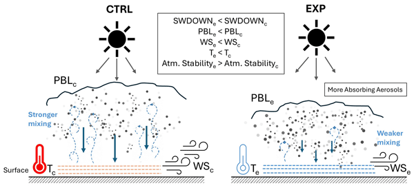
L462-466: It is good to include a schematic of the processes, but I feel that some of the literature on the topic should be acknowledged. For instance Ding et al. (2016) describes the enhanced air pollution through aerosol-PBL interactions due to absorbing aerosols and shows a similar schematic. And the Sharma et al. (2023) paper mentioned previously is highly relevant for this study.
Ding, A. J., X. Huang, W. Nie, J. N. Sun, V.-M. Kerminen, T. Petäjä, H. Su, Y. F. Cheng, X.-Q. Yang, M. H. Wang, X. G. Chi, J. P. Wang, A. Virkkula, W. D. Guo, J. Yuan, S. Y. Wang, R. J. Zhang, Y. F. Wu, Y. Song, T. Zhu, S. Zilitinkevich, M. Kulmala, and C. B. Fu (2016), Enhanced haze pollution by black carbon in megacities in China, Geophys. Res. Lett., 43(6), 2873-2879, doi: https://doi.org/10.1002/2016GL067745.
L471-474: Are these simulations different from what was used in sections 3.1-3.4?
L474-476: What is the reason for showing domain 1 results? Unless the point is to discuss differences in results between resolutions, which I sense it is not, then I would replace Figure 9 with Figure S5 showing the domain 2 results. They look anyway very similar.
L480-482: I cannot see that Table 2 shows any of this
L488-489: It does not look like the changes due to RI of BC/OC are twice as high in November. Maybe close to twice as high as in October, but not for the other months.
L496-497: Again, it would be useful to know if one-way or two-way nesting was used. If two-way nesting, then the results in domain 1 and 2 should be the same.
L500-506: I suggest discussing RMSE instead of the mean bias. If it is as in section 3.2, different periods of overestimation and underestimation compensate, which leads to a very small mean bias. The RMSE accounts for this, and in Table S9 it shows that the RMSE reduction is not nearly as large as the reduction in mean bias.
L522: Remove “thus”
L524-525: I do not think the surface temperature change is a main driver here. Since the modifications to the refractive indices make the aerosols more absorbing, I would expect the vertical temperature profile to change and make the atmosphere more stable. This would involve weaker winds and shallower boundary layer. See for instance the Ding et al. (2016) paper mentioned previously or Stjern et al.:
Stjern, C. W., Ø. Hodnebrog, G. Myhre, and I. Pisso (2023), The turbulent future brings a breath of fresh air, Nature Communications, 14(1), 3735, doi: 10.1038/s41467-023-39298-4.
L582-584: Should remove “significantly” – it is not shown that EXP5 performs significantly better than CTRL. And where do the 25-37 W m-2 bias reduction numbers come from? Table S9 shows only a small reduction. Same with the ~80 W m-2 bias reduction, where is that from?
L584-589: It looks like these are the maximum changes during the extreme event no. 1, so the improvements appear a bit overstated, in my opinion.
Citation: https://doi.org/10.5194/egusphere-2026-1100-RC2 - AC1: 'Reply on RC1', Sumit Kumar, 09 Jul 2026
Peer review completion
Journal article(s) based on this preprint
Viewed
| HTML | XML | Total | Supplement | BibTeX | EndNote | |
|---|---|---|---|---|---|---|
| 765 | 360 | 66 | 1,191 | 150 | 64 | 61 |
- HTML: 765
- PDF: 360
- XML: 66
- Total: 1,191
- Supplement: 150
- BibTeX: 64
- EndNote: 61
Viewed (geographical distribution)
| Country | # | Views | % |
|---|
| Total: | 0 |
| HTML: | 0 |
| PDF: | 0 |
| XML: | 0 |
- 1

Gaurav Govardhan
Sreyashi Debnath
Avinash N. Parde
Sandeep Wagh
Jimy Dudhia
Sachin D. Ghude
The requested preprint has a corresponding peer-reviewed final revised paper. You are encouraged to refer to the final revised version.
- Preprint
(1502 KB) - Metadata XML
-
Supplement
(647 KB) - BibTeX
- EndNote
- Final revised paper
Referee comment on egusphere-2026-1100
“Improving aerosol–radiation interaction feedback in AIRWISE operational system”
General comments
This manuscript studies aerosol–radiation interactions in the AIRWISE (WRF‑Chem) operational system over Delhi. The authors update aerosol complex refractive indices (RI) and run a control simulation and sensitivity experiments for Oct 2023–Jan 2024. They show impacts on SWDOWN, near-surface meteorology, PBL height, and PM2.5, and they compare SWDOWN with WiFEX observations at IGI airport.
Overall, I do not see a major conceptual problem in the approach. The study is rather straightforward (control run + sensitivity runs with changed optical assumptions), and results are mostly plausible. However, I am not fully convinced about the novelty level for ACP, but this is editor’s decision. Several key parts need clearer description and more careful wording of conclusions.
Main comments
1) “Region-specific” refractive indices – please justify or reword
The manuscript repeatedly calls the modified RI values “region-specific”. However, I did not find a clear explanation why these values are truly specific to Delhi. Many of the changes look like more general literature updates (e.g., updated BC imaginary part, and discussion of absorbing OC/brown carbon at shorter wavelengths), rather than values specifically suitable for aerosol composition in Delhi or based on measurements (use of Mishra and Tripathi, 2008 for dust, is perhaps an exception). Please clarify your motivation to use “region-specific” here.
2) Hygroscopic growth / aerosol water uptake is not described in Methods, but it is critical information
I did not find a clear description in the model setup section about aerosol hygroscopic growth / aerosol water uptake and how it is treated in the optical calculations. This is important because aerosol optical effects depend not only on RI and size distribution, but also strongly on RH-driven water uptake (wet size, wet RI, and thus extinction/scattering).
You mention in the Results that the model has difficulty with fog because of RH bias, and you link this to underestimated hygroscopic growth and to PM2.5 underestimation. I think this statement is too vague and may be confusing. If your model PM2.5 includes aerosol water mass (wet PM2.5), then low RH can directly reduce PM2.5 through reduced water uptake. But I assume, and it should be clearly stated, that you compare dry PM2.5 mass. Then, if “underestimated hygroscopic growth” is used to explain lower dry mass, I assume you mainly mean that fog/high RH conditions increase secondary aerosol formation / partitioning and the model misses that process when RH is too low. This should be clarified and explained in more detail.
3) Radiation observations in Fig. 2 are too vaguely described (“observations”, “net radiometer”)
In Fig. 2 the observational curve is labelled only as “observations”, and in the text you mention “net radiometer”. This is ambiguous because a “net radiometer” can mean a single-output net radiation instrument (net all-wave), or a 4-component system that provides downward and upward SW and LW components separately.
Please add some relevant instrument metadata (type/model if possible) and specify the variable used in the comparison. Also, please state the spectral range of the SW sensor. Some pyranometers do not cover the full solar range, and this can create a small systematic offset when comparing to modeled broadband SWDOWN (even a couple percent).
4) Time axis and diurnal mismatch. Fig. 2 uses IST (“Local Time”). It is normal that the SWDOWN peak is not exactly at 12:00 IST because IST is a national time reference and local solar noon in Delhi is shifted. This is not a problem. However, more important is the model–observation mismatch pattern: it looks like the model is too high in the morning (until near noon), while agreement is better in the afternoon. Please discuss possible causes. From your paper, I assume that morning fog / cloudiness is perhaps the key reason, even now when you tried to have clear-sky cases only. But is it true or are there other reasons that would be useful information for the readers? What was the time window of ground-based measurement, hourly? Could the reason be then as simple as the time stamp for hourly mean being not fully representative for hourly mean, which would mean different impact before and after noon (when SZA is decreasing, and increasing, respectively).
5) Emissions year / representativeness
In Methods, anthropogenic emissions are from EDGAR-HTAP v2.2 (2010) and you mention “fine-gridded emissions over Delhi-NCR”. Please clarify what this refinement is (source/year/scaling). This is relevant for aerosol composition and PM2.5 interpretation in 2023–24
The phrase “position vector of the particle” (line 69) is confusing in this context. What did you mean: “spatial location (grid cell)” rather than something about particle microphysics? Please reword to avoid misunderstanding.
The statement “hematite … with global average of 6.85% (Goudie, 1978)” (line 80), and other similar %-numbers there, is unclear. Please specify % of what (mass fraction of dust? fraction of iron oxides? something else). As written, it is ambiguous.
“The AOD at specific wavelengths, such as 400 and 600 nm, is derived using the Ångström exponent formula” (line 72) I assume 400, 600 are not derived using AE, since these belong to those four shortwave radiation bands. Please be more specific here.
“… in which we have removed the cloud cover (set > 0.1) in the model along with the foggy hours …” (line 301) Please clarify what “cloud cover >0.1” means (units/definition) and how cloud cover is estimated (ceilometer method?). Please give the needed.