
the Creative Commons Attribution 4.0 License.
the Creative Commons Attribution 4.0 License.
 | 04 Feb 2026
Evidence for the impact of fire activity on daily variations of IASI mid-tropospheric CO2 anomalies at 8–11 km
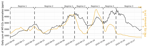
Abstract. Biomass burning is a major, highly variable source of atmospheric CO2, but its impact on the free troposphere remains difficult to quantify because of uncertainties in injection heights and transport. In the tropics, intense fires can trigger pyroconvective plumes that loft combustion products to the mid- and upper troposphere. However, most fire emission inventories and global CO2 inversions still assume simplified vertical distributions of CO2 emitted by fires. Weighted columns of CO2 retrieved from remote sensing instruments that are sensitive to such high-altitude enhancements can inform of such dynamics. Here we combine mid-tropospheric CO2 (MT-CO2) retrievals from three IASI instruments with GOES-16 observations of Fire Radiative Energy (FRE) to link daily MT-CO2 anomalies observed by IASI at 8–11 km altitude to South American fire activity during the 2020 burning season, while accounting for long-range horizontal transport of anomalies. From August–October 2020, about 66 % of the detected anomalies originate from long-range or unknown sources and are discarded. For the remaining anomalies attributed to local fires, 72 h back trajectories do intersect with at least one active fire for 75 % of them. Their daily sum co-varies strongly with FRE, with the ratio between the two depending on the dominant horizontal transport regime. A comparison with CAMS IASI-weighted CO2 fields shows that model fails to reproduce both the amplitude and structure of the observed anomalies. Overall, our results demonstrate that IASI MT-CO2 anomalies carry an observational fingerprint of tropical fire activity.
-
Notice on discussion status
The requested preprint has a corresponding peer-reviewed final revised paper. You are encouraged to refer to the final revised version.
-
Preprint
(1651 KB)
-
Supplement
(95 KB)
-
The requested preprint has a corresponding peer-reviewed final revised paper. You are encouraged to refer to the final revised version.
- Preprint
(1651 KB) - Metadata XML
-
Supplement
(95 KB) - BibTeX
- EndNote
- Final revised paper


Journal article(s) based on this preprint
Interactive discussion
Status: closed
- RC1: 'Comment on egusphere-2025-6426', Anonymous Referee #1, 18 Feb 2026
-
RC2: 'Comment on egusphere-2025-6426', Anonymous Referee #2, 27 Mar 2026
This is a very nice study on the pyroconvection signal of CO2 in the upper troposphere using IASI observations. The study focuses on the 2020 fire season in South America which is characterised by intense fires and the availability of 3 IASI instruments. To assess the impact on the global carbon cycle it would be nice to have extended this study to tropical Africa which as the paper mentions is the largest contributor to fire emissions. The results demonstrate the potential of IASI to assess the inversion model capabilities for representing pyroconvection, as well as potentially long-range transport. The paper is well written and the methodology is well illustrated.
Minor comments to be addressed:
1. Because IASI is only sampling the upper troposphere, the CO2 fire anomalies will be associated with pyroconvection. It might be useful to clarify this in the title and abstract. It would also be useful to mention how common is pyroconvection and what is the contribution to the global budget of biomass burning in order to put this study in the context of the global carbon cycle. This should be included in the introduction.
1. In the abstract the CAMS CO2 fields are mentioned without specifying whether it is the CAMS inversion or the CAMS IFS analysis. This is later clarified, but it should be good to specify this in the abstract to avoid confusion. The CAMS inversion has a low resolution and no representation of injection height for the fire emissions, while the CAMS IFS CO2 forecast has has resolution and a representation of the fire injection height. It would have been interesting to compare the two products with the IASI anomalies.
2. I am not convinced about the use of the sum of the CO2 anomalies in ppm, as concentrations or dry molar fractions are not supposed to be integrated without previous conversion to mass.
3. Line 9: It would be useful to be consistent with the units throughout (e.g. PgC or GtCO2).
4. Lin 43: The claim that spaceborne retrievals of partial columns in the upper-troposphere and total column provide information on the vertical distribution is a bit far fetched because it does not allow to separate strong atmospheric signals coming from the near-surface or the stratosphere.
5. Line 53: The sentence "a substantial body of work has used satellite observations to track fire-emitted but mostly using CO observations." is not clear/complete.
6. The influence of atmospheric chemistry is not addressed in this paper. What is the influence of atmospheric chemistry (i.e. chemical production of CO2 from CO oxidation) on CO2 anomalies in the upper troposphere detected by IASI? Could chemical production also change the amplitude of the plumes in the circular transport scenario and therefore contribute to the lower correlation coefficient with FRE?
7. There is a missing full stop "." in line 81
8. Are the IASI IR retrievals affected by aerosols from biomass burning?
9. Line 92: Typographical error: 180oS and 180oN should be 180oW and 180oE.
10. Line 180: ERA-5 provides hourly data. Why are the hourly winds from 3-hourly fields?
11. Line 179: Shouldn't the back-trajectories start from a range of altitudes representing the layer sampled by IASI rather than the peak altitude?
12. Line 399: Misspelling "extant"
13: Line 405 & lines 435-439: Even with the inclusion of pyroconvection, the global inversion models might have too coarse resolution (both in vertical and horizontal dimensions) to be able to represent the CO2 anomalies in the upper troposphere. In order to link the effect of ignoring the pyroconvection process, it would be useful to understand what is the proportion of intense fires with pyroconvection and therefore the impact on the global budget.
Citation: https://doi.org/10.5194/egusphere-2025-6426-RC2 -
AC1: 'Final response', Victor Bon, 28 Jun 2026
We thank both referees for their careful and constructive reviews, which have substantially sharpened the physical interpretation of the results and improved the clarity of the manuscript. We respond to each referee in turn. Referee comments are shown in italic; our responses follow, with a final “Changes” note indicating the corresponding revisions to the manuscript. Where a comment from the second referee overlaps with one already addressed for the first, we answer it in its own right and refer back to the earlier response. Manuscript line numbers refer to the discussion preprint.
Response to Referee 1:
- RC1.1 (L90–96): Background assumptions and “background fires”
Referee comment: These kind of assumptions need to be made, but it would be nice to have a sensitivity analysis where you show how your results vary, had you made different assumptions. Do the “background fires” also lead to anomalies or only the ones that are larger than those “regular” fires? It will be mostly the larger ones that have pyroconvection and thus relevant for your work. It is worthwhile to know whether those are the norm or the exception.
Response:
We thank the referee for this point, which has two facets: the robustness of the background construction, and whether “background” fires (rather than only the most intense ones) generate the anomalies we analyse. We address them in turn.
The essential property of our background is that it is computed as a zonal median over an entire latitude band (±2°, spanning 180°W–180°E, land and ocean indistinctly). Each band therefore mixes the comparatively few, localised regions strongly affected by fires with the much larger fraction of the band, in particular the oceans, that is less affected. The median of such a band is consequently close to the regional, fire-free background, and a fire-affected region stands out as a positive departure from it. This is the basis on which fire emissions can be distinguished from the fire signal at all, and it underlies our answer below.
Two assumptions enter this construction: the size of the spatiotemporal pool (±3-day, ±2° latitude) and the interquartile-range (IQR) outlier filter. Both were set deliberately to keep the baseline from tracking the pervasive seasonal fire activity. The pool size results from a sensitivity test balancing two failure modes: a narrower window leaves too few clear-sky observations per estimate, particularly at the edges of the tropical domain where IASI coverage is sparse, while a wider window incorporates observations from meteorologically distinct conditions and from different phases of the fire season, biasing the baseline. The ±3-day / ±2° choice yields pools of several thousand to several tens of thousands of observations while remaining narrow enough to resolve the meridional CO₂ gradient and the seasonal cycle. The IQR/Tukey filter then prevents the extensive fire season from inflating the background: fire-contaminated values populate the high-concentration tail of each pool, and the upper Tukey fence removes them before the median is taken. On a representative September case-study pool, the filter excludes 4.9% of observations (all in the high tail) and retains 95.1%, so the resulting baseline reflects the near-fire-free condition rather than the seasonally elevated one. These choices were established through explicit sensitivity tests (for the temporal window we tested ±1 day, ±3 days, ±1 week and ±1 month, and for the spatial window fixed bands and then moving bands) together with analyses of the anomaly distribution and of the false-detection rate used to set the threshold.
Against this near-fire-free baseline, every fire produces some positive perturbation, but only a small, intense subset survives into the retained anomaly population, for a physical reason. Using the IASI averaging kernels we verified that a CO2 enhancement confined below 4 km cannot produce a mid-tropospheric anomaly at our detection level: even a uniform +20 ppm filling the entire 0–4 km boundary layer yields a retrieved signal of only ~1.5 ppm, and a +10 ppm perturbation yields ~0.7 ppm, both well below the 4 ppm threshold. A retained anomaly therefore requires emissions lofted above ~4 km by active convective or pyroconvective transport. To keep the article concise we report these in summary form; the full sensitivity analysis (distribution fit, false-detection-rate curve, kernel-propagation experiment) is available and we are happy to include it as a Supplement if the editor prefers.
The “regular” background fires whose smoke stays in the boundary layer do not produce retained anomalies; the retained population is, by construction, the exception (the intense, vertically efficient fires) which is exactly the population the referee identifies as relevant. However, since the pyroconvection is a complex interplay between fire intensity, atmospheric instability, types of fires etc, we see that the frequency of the fires that produce pyroconvection evolves during the fire season. The frequency of this population and its bearing on the global budget are addressed in our response to RC2.1.
Changes: The sentence introducing the dynamic background in Sect. 2.1 has been expanded to state explicitly that it is a zonal median over a latitude band spanning land and ocean, so that fire-affected regions stand out against a near-fire-free baseline. A sentence has been added to Sect. 2.1 making explicit that the 4 ppm threshold selects, by construction, emissions lofted to the free troposphere. [Lines 90–96 → new lines 130–135.]
- RC1.2 (L219): Matching anomalies to specific fire detections
Referee comment: Given that you more or less know when CO₂-concentrations were enhanced and what the atmospheric transport was, are you able to more closely match anomalies with actual active fire detections (with some uncertainty)? So instead of investigating whether the back-trajectory intersected with fire detections, actually say with which fire detections? And would the match then still be 75%? This could be relevant for follow-up work that could take advantage of linking vegetation types with plumes, or understanding how pyroconvection changes over the time of day.
Response:
We first note that the analysis already retains specific space–time fire encounters, not merely a binary “intersected a fire.” For each source-attributed anomaly, the collocation is performed against 1°×1° hourly aggregations of GOES-16 FRP along the trajectory, and the last such encounter (its location and FRP) is shown in Fig. 4G–I. The 75% reported at L278 is precisely this collocation rate at 1° hourly resolution, i.e. the fraction of retained anomalies for which at least one specific space–time fire aggregation is identified along the back-trajectory.
We deliberately collocate at 1° hourly rather than at the native 2 km pixel and instantaneous time, for two physical reasons: the mid-tropospheric injection is not located directly above the surface FRP pixel, since the air parcel is sheared horizontally between the surface and the 8–11 km injection level during convective ascent and subsequent transport; and the trajectory computation and driving reanalysis carry their own positional uncertainty. The 1° hourly scale is chosen to absorb both, so matching at finer resolution would reduce the apparent agreement for these reasons rather than because the underlying fire–anomaly link is weaker.
What is not robust, in most cases, is the attribution of an anomaly to a single source fire: a given anomaly is typically collocated with several distinct 1° hourly fire aggregations, and pyroconvective injection depends on several co-varying parameters (atmospheric instability, fuel moisture, FRP, burning duration), so without an explicit per-fire injection-probability model the candidate fires cannot be ranked reliably. We did attempt to rank candidate contributors by combining each FRP aggregation with a CAPE/CIN-based convective indicator, but these results require further analysis and fall outside the scope of the present paper, whose aim is to establish the link between daily fire activity (FRE) and the MT-CO₂ anomaly sum. We agree this is a promising avenue, for linking vegetation and plume types and for studying the diurnal evolution of pyroconvection, and now identify it explicitly as future work.
Changes: A future-work sentence has been added to the Conclusion identifying per-fire attribution, vegetation/plume-type linkage and diurnal-pyroconvection study as directions enabled by a CAPE/CIN-based convective indicator. [New sentence at lines 491–495.]
- RC1.3 (L179): 1° wind resolution
Referee comment: 1 degree is very coarse and there are higher spatial resolution wind fields available. It would improve the quality of the study.
Response:
At the outset of the study we qualitatively compared back-trajectories driven by the native ERA5 winds (~0.25°) against the 1° fields used here and found no appreciable difference in trajectory paths, at substantially higher computational cost. Since the FRE and wind fields share the same 1° grid, this resolution is also internally consistent for the source–receptor analysis.
Changes: None.
- RC1.4 (L184): Points north of 35°N
Referee comment: How about points north of 35N?
Response:
South American fire sources lie in the Southern-Hemisphere tropics and subtropics. At 250 hPa over a 72h window, the upper-level flow and the position of the ITCZ make transport reaching 35°N very rare, so a northern counterpart to Filter 1 is not required for the period and region studied.
Changes: The corresponding statement in Sect. 3.1 has been clarified. [Line 206-209.]
- RC1.5 (L314): Why recirculation periods still appear as anomalies
Referee comment: For this period the CO₂:FRE ratio is very high, partly due to recirculation. I don’t fully understand why these periods still show up as anomalies; they are not lofted anymore due to pyroconvection and CO₂-concentrations become more uniform probably.
Response:
As set out in our response to RC1.1, the background is a global zonal median over a ±2° latitude band (180°W–180°E). Hence, even when recirculation makes CO₂ more uniform over South America, the recirculating region remains elevated relative to the global zonal background, which is dominated by the fire-free remainder of the band, including the oceans, and is still flagged as an anomaly. The large anomaly sum during these periods reflects the accumulation of CO₂-enriched air from consecutive FRE peaks and the longer mid-tropospheric residence time imposed by circular transport; nonetheless, the day-to-day variations of the sum continue to track FRE. A plausible additional contributor is the seasonal increase in atmospheric instability, consistent with observed end-of-season increases in injection efficiency (Gonzalez-Alonso et al., 2019): late-season fires may loft material at lower intensities than earlier in the season, although this cannot be confirmed without a transport model that explicitly resolves convection and pyroconvection.
Changes: None.
- RC1.6 (L369): Controls beyond FRE; future CO–CO₂ synthesis
Referee comment: “…the amplitude of the atmospheric response is not determined by FRE magnitude alone, but also by fuel type, size, density, moisture content, and local meteorology.” I feel this is crucial and would appreciate more text on what can be done in the future and how, for example, studies focusing on CO and CO₂ can be merged here to improve our understanding of fires, their emissions, and their fate in the atmosphere.
Response:
We agree and have expanded this discussion. We now elaborate on the controls of injection amplitude beyond FRE (fuel load and type, moisture content, combustion phase, and the meteorological modulation of injection efficiency through atmospheric instability), and on the prospects for a multi-species approach: combining the co-emitted CO and CH4 also retrieved from IASI would allow joint constraints on injection heights and on emission types across tropical biomes, linking the strong, easily tracked CO signal to the weaker CO2 anomalies studied here.
Changes: The relevant Discussion paragraph has been expanded with the controls on injection amplitude beyond FRE and the multi-species (CO + CH4) prospect, and the corresponding sentence in the Conclusion strengthened. [Lines 392–397.]
- RC1: Technical corrections
All technical corrections have been adopted:
- L16: “active fire” → “active fire detection” where it refers to FRP observations.
- L23 (and reference list): “Ipcc” → “IPCC”.
- L25: Andreae (2019) added for the CO₂/CO/CH4 emission split (the percentages are consistent with the emission factors compiled there); the Pg C figures remain supported by van der Werf et al. (2017).
- L27–29: carbon figures now reported consistently in Pg C (see also RC2.4).
- L35: Langenfelds et al. (2002, GBC) added for the interannual fire–CO₂ growth-rate link; sentence completed to “…track fire-emitted gas…” (see also RC2.6).
- L67: a brief gloss locating the Pantanal (the world’s largest tropical wetland, spanning Brazil, Bolivia and Paraguay) added.
- L81: missing full stop inserted (see also RC2.8).
- L100: “biomass burnings” → “biomass burning regions”.
- L102: “values” → “anomalies”.
- L148: “maps” → “emission fields”.
- L198: “5×5” set with the cross symbol (×).
- L291, L299: “anomaly” → “anomalies”.
- L298: regime adjectives lowercased in running prose, while defined labels (e.g. “Regime 1 (Longitudinal)”) retain their capitalisation.
- L357: “Discussions” → “Discussion”.
- L405: “mandatory” → “crucial” (see also RC2.14).
- Figure 3 re-exported at higher resolution; Figure 6 re-exported at higher resolution.
Response to Referee 2
- RC2.1: Pyroconvection in title and abstract; how common it is; contribution to the global budget
Referee comment: Because IASI is only sampling the upper troposphere, the CO₂ fire anomalies will be associated with pyroconvection. It might be useful to clarify this in the title and abstract. It would also be useful to mention how common is pyroconvection and what is the contribution to the global budget of biomass burning in order to put this study in the context of the global carbon cycle.
Response:
We have revised the title to make the pyroconvective interpretation explicit: “Evidence for the impact of fire activity on daily IASI mid-tropospheric CO₂ anomalies at 8–11 km over South America: a pyroconvective fingerprint.”
How common is pyroconvection, and how does that bear on the budget? It is the exception in fire count but dominates the free-tropospheric flux. Amazon climatologies find that only ~3–20% of fires inject smoke into the free troposphere (Gonzalez-Alonso et al., 2019), consistent with plume-rise modelling (Rio et al., 2010; Freitas et al., 2007). This fraction is strongly skewed toward the most intense fires: free-tropospheric plumes carry FRP an order of magnitude higher than boundary-layer-trapped plumes (Val Martin et al., 2010).
However, we note two caveats now stated in the manuscript. Pyroconvection is not a fixed property of a fire but a convolution of intensity, size, fuel load/type and moisture, combustion phase, and atmospheric instability that evolves through the season; a single “fraction of fires with pyroconvection” conflates these and is not a transferable statistic, which is why we frame budget relevance through the injection fraction rather than a fire count. Consistently, the free-tropospheric injection fraction is not constant but rises through the season as atmospheric stability decreases, from ~3–20% over the Amazon in the mean to ~15–40% late in the season (Gonzalez-Alonso et al., 2019), meaning fires need progressively less energy (FRE) to reach the free troposphere as the season advances. Finally, 2020 was an exceptionally intense South American season (Silveira et al., 2022; Garcia et al., 2021), so the lofted signal and its detectability by IASI are likely larger than in a climatologically average year.
On the global-budget context, although the pyroconvectively lofted fraction is a small part of this total, its budget relevance lies in the fact that the vertical placement of fire emissions is the least observationally constrained element of the biomass-burning contribution to the carbon cycle: global inversions have historically relied on prescribed injection profiles and only recently began incorporating satellite-derived injection heights. By showing that IASI MT- CO2 anomalies carry an observable fingerprint of this lofted fraction, our study provides a direct constraint on precisely the part of the ~2.1–2.2 Pg C yr⁻¹ fire flux that models place most uncertainly in the vertical.
Changes: The title has been revised to make the pyroconvective interpretation explicit. A paragraph has been added to the Introduction on the frequency of pyroconvection and the link to global carbon budget. [Lines 41–48.]
- RC2.2: CAMS product identity in the abstract; comparison of inversion vs. assimilating product (EGG4)
Referee comment: In the abstract the CAMS CO₂ fields are mentioned without specifying whether it is the CAMS inversion or the CAMS IFS analysis. The CAMS inversion has a low resolution and no representation of injection height for the fire emissions, while the CAMS IFS CO₂ forecast has high resolution and a representation of the fire injection height. It would have been interesting to compare the two products with the IASI anomalies.
Response:
We have specified the product in the abstract: the primary comparison uses the CAMS global inversion-optimised CO2 product (v23r1; Chevallier, 2023), not the IFS forecast/analysis. The inversion optimised is the appropriate primary product for two reasons. First, it is constrained by surface in-situ observations and is independent of IASI, so the comparison against IASI MT-CO2 anomalies is not self-referential. Second, it provides globally consistent fluxes and 3-hourly concentrations but no explicit representation of fire-driven pyroconvective injection, which makes it the correct null test: if a surface-constrained, observationally optimised inversion still fails to reproduce the 8–11 km anomalies, the discrepancy isolates a missing vertical process rather than a surface-flux error (Fig. 7).
Following the referee’s suggestion, we additionally compared the IASI anomalies against a product that does represent fire injection. The high-resolution CAMS global GHG forecast, which carries an injection-height representation, has a temporal coverage beginning in March 2024 and cannot be applied to the 2020 period studied here. We therefore turned to the CAMS EGG4 greenhouse-gas reanalysis, which covers 2020 and distributes GFAS biomass-burning emissions in the vertical using Plume-Rise-Model injection heights; this product however assimilates IASI CO₂ observations, including those used in this study, so the comparison is not fully independent. It is now included as Fig. 8 and discussed in Sect. 5.
What we see now is that EGG4 also fails to reproduce the mid-tropospheric anomalies, and for a representative day (1 September 2020) the figure isolates why. Its surface CO₂ field (Fig. 8d) is in fact richer and more fire-resolved than the inversion’s, with enhancements exceeding 100 ppm over southern Amazonia and the Pantanal that closely track the FRE field (Fig. 8c), a direct consequence of EGG4 distributing GFAS fire emissions at the surface. Yet the IASI-weighted mid-tropospheric field (Fig. 8b) is essentially indistinguishable from that of the IASI-independent inversion and shows none of the coherent 8–11 km anomalies seen by IASI (Fig. 8a). Two conclusions follow. First, although EGG4 assimilates IASI CO₂, the assimilation leaves no visible imprint on the mid-tropospheric field, consistent with the large, fire-driven departures being down-weighted or rejected by the variational quality control. Second, and independently, the fire signal that EGG4 clearly represents at the surface does not reach the free troposphere: the GFAS Plume-Rise-Model injection heights are known to be biased low (Rémy et al., 2017; Tang et al., 2022), so emissions are deposited too low in the column and never populate the 8–11 km layer. The two comparisons are thus complementary: the IASI-independent inversion provides the clean null test, while EGG4 shows that even an injection-height-aware, IASI-assimilating product does not capture the anomalies, indicating that the limitation lies in the fidelity of the represented injection process rather than its mere absence.
Changes: The CAMS inversion-optimised product (v23r1) is now named explicitly in the abstract, noting that it is sampled with the IASI vertical weighting. A new figure (Fig. 8) and an accompanying Discussion paragraph have been added, comparing the IASI MT-CO₂ anomalies against the CAMS EGG4 reanalysis (surface vs. mid-troposphere). [Fig. 8 and Discussion paragraph at lines 438–465.]
- RC2.3: Summing CO₂ anomalies in ppm without conversion to mass
Referee comment: I am not convinced about the use of the sum of the CO₂ anomalies in ppm, as concentrations or dry molar fractions are not supposed to be integrated without previous conversion to mass.
Response:
We agree that mole fractions are not formally additive across grid cells of differing air mass, and we have clarified that the summed anomaly is used only as a relative, temporal co-variability index and not interpreted as a CO₂ mass or flux. The referee’s underlying concern is whether moving to a proper mass formulation would change our conclusions. It does not, for the following reasons.
Converting an individual anomaly from a mole fraction (ppm) to a mass (tonnes of CO₂) requires multiplying by the air mass of the sounded volume, set by the thickness of the contributing layer and the horizontal footprint of the observation. For our IASI dataset both are effectively constant across the retained sample: the footprint varies only weakly because we restrict the analysis to a limited solar-zenith-angle range, and the layer thickness varies only slightly with latitude through the IASI averaging kernels, within the same order of magnitude across our narrow, day-to-day-stable latitude band. The ppm→mass conversion is therefore, to good approximation, a near-constant multiplicative factor across both the spatial sum and from one day to the next; multiplying the daily sum by such a factor rescales the curve but leaves its temporal evolution , and hence the day-to-day tracking of FRE and the per-regime correlation coefficients, the only quantities we draw conclusions from, unchanged.
We have verified this directly: converting the CO₂ anomaly sum to a mass and comparing it against FRE in equivalent mass units (via the GFAS emission-coefficient methodology) leaves both the temporal variations and the regime-dependent correlations essentially identical to the ppm-based analysis. We have chosen not to replace the figures with the mass-converted version, because the conversion is a near-constant linear rescaling that adds nothing to the central message; presenting a mass-based sum would additionally require converting FRE into the same units and detailing the full GFAS methodology; and the manuscript is already dense. We are happy to provide the mass-converted comparison as a Supplement if the editor would find it useful.
Changes: None.
- RC2.4 (L9): Unit consistency
Referee comment: It would be useful to be consistent with the units throughout (e.g. PgC or GtCO₂).
Response:
We have harmonised the manuscript to use Pg C throughout, converting the Gt CO₂ figures accordingly.
Changes: Carbon-flux figures standardised to Pg C throughout (consistent with RC1, L27–29). [Affects the abstract (L9) and the Introduction.]
- RC2.5 (L43): Partial columns and the “vertical distribution” claim
Referee comment: The claim that spaceborne retrievals of partial columns in the upper troposphere and total column provide information on the vertical distribution is a bit far-fetched because it does not allow to separate strong atmospheric signals coming from the near-surface or the stratosphere.
Response:
The referee is right, and we have rephrased. A single partial column provides one weighted layer value rather than a vertical profile, and cannot by itself separate near-surface from stratospheric contributions. Our intended point was that partial-column retrievals isolate the contribution of a specific layer (here the mid-troposphere), and that combining columns with differing vertical sensitivities constrains the vertical distribution.
Changes: L43 has been rewritten as: “…are sensitive to different parts of the atmospheric column. While a single partial column does not resolve a full vertical profile, it isolates the contribution of a specific layer (here the mid-troposphere); combining columns with differing vertical sensitivities further constrains the vertical distribution of CO₂.” [Line 51-55.]
- RC2.6 (L53): Incomplete sentence
Referee comment: The sentence “a substantial body of work has used satellite observations to track fire-emitted but mostly using CO observations” is not clear/complete.
Response:
Corrected: the missing word was “gas”. The intended meaning is that most studies tracking fire emissions through transport rely on CO, the easiest tracer owing to its strong signal relative to the background.
Changes: L65 completed to “…track fire-emitted gas…” and lightly rephrased for clarity (see also RC1.6).
- RC2.7: Influence of atmospheric chemistry (CO → CO₂)
Referee comment: What is the influence of atmospheric chemistry (i.e. chemical production of CO₂ from CO oxidation) on CO₂ anomalies in the upper troposphere detected by IASI? Could chemical production also change the amplitude of the plumes in the circular transport scenario and therefore contribute to the lower correlation coefficient with FRE?
Response:
Chemical production of CO₂ from CO oxidation is negligible at the timescale of our analysis. The tropospheric lifetime of CO is of order one to two months, so over a 72 h trajectory at most a few percent of the plume CO is oxidised, almost all of it to CO₂. With fresh-plume CO enhancements of order 100 ppb, this yields of order a few ppb of CO₂, of order 0.1% of the multi-ppm (≥4000 ppb) anomalies we analyse. On the referee’s specific point, chemical production in aged air masses would act in the same direction as the recirculation and accumulation we invoke for the circular regime, but it is several orders of magnitude too small to affect the amplitude of the anomalies or the correlation coefficients; the regime-dependent residence time is the dominant control.
Changes: None.
- RC2.8 (L81): Missing full stop
Referee comment: There is a missing full stop in line 81.
Response:
Corrected.
- RC2.9: Sensitivity of IASI IR retrievals to biomass-burning aerosols
Referee comment: Are the IASI IR retrievals affected by aerosols from biomass burning?
Response:
Aerosols may also impact the IASI signal, but two factors limit any effect on our results. However, only clear-sky observations are considered in this study, so that coarse aerosols as well as clouds have already been filtered out using a dedicated screening procedure (Capelle et al., 2018). We therefore consider that our signal may only be affected by residual aerosols, which cannot plausibly generate the spatially coherent, FRE-correlated anomalies analysed here.
Changes: A statement on aerosol sensitivity has been added to Sect. 2.1, noting that coarse aerosols and clouds are removed by the clear-sky screening of Capelle et al. (2018). [Lines 100–103.]
- RC2.10 (L92): Typographical error
Referee comment: 180°S and 180°N should be 180°W and 180°E.
Response:
Corrected, here and in the background definition (the longitude range is 180°W–180°E).
- RC2.11 (L180): Why 3-hourly ERA5 winds
Referee comment: ERA-5 provides hourly data. Why are the hourly winds from 3-hourly fields?
Response:
We used 3-hourly ERA5 fields because a qualitative comparison showed trajectories with no appreciable difference from those driven by hourly winds, at a large reduction in computational cost. LAGRANTO interpolates the fields in time during the integration, so sub-3-hourly variability has negligible effect at the daily, regional scale of this study.
- RC2.12 (L179): Initialising from a layer rather than the peak altitude
Referee comment: Shouldn’t the back-trajectories start from a range of altitudes representing the layer sampled by IASI rather than the peak altitude?
Response:
In principle, initialising over the full sensitive layer would be more complete. However, our attribution is a horizontal source–receptor problem, and over a 72 h window the large-scale flow that governs horizontal transport is vertically coherent across the IASI-sensitive layer, so initialising at a representative level rather than integrating over the layer does not materially change which fires are intersected or the filtering outcome. The chosen level (250 hPa) is representative of the peak sensitivity at the subtropical latitudes where most of the retained anomalies occur (Fig. 1). A full layer treatment would also require a rule for combining the resulting ensemble of trajectories per anomaly, adding substantial complexity and cost for negligible benefit given the daily, regional scope of the study.
- RC2.13 (L399): Misspelling
Referee comment: Misspelling “extant”.
Response:
Corrected to “extent” (here and in the Fig. 7 discussion paragraph).
- RC2.14 (L405 & L435–439): Proportion of pyroconvective fires; model resolution; budget impact
Referee comment: Even with the inclusion of pyroconvection, the global inversion models might have too coarse resolution (both vertical and horizontal) to represent the CO₂ anomalies in the upper troposphere. In order to link the effect of ignoring the pyroconvection process, it would be useful to understand what is the proportion of intense fires with pyroconvection and therefore the impact on the global budget.
Response:
We thank the referee, whose comment helped us sharpen the broader significance of the study. On resolution, the referee’s premise is correct, and the revised manuscript now demonstrates it. Global inversions cannot (for now) intrinsically resolve the sub-grid-scale convective dynamics that loft fire emissions; injection must be prescribed or parameterized (Veira et al., 2015; Paugam et al., 2016), and the parameterizations in operational use are known to underestimate the highest injections, placing most emissions near the boundary layer (Rémy et al., 2017; Tang et al., 2022). Our new comparison against EGG4 (Fig. 8) makes this concrete: a product that does carry GFAS injection heights still reproduces the surface anomaly but not the 8–11 km signal, exactly the pattern expected from low-biased injection. Adding a pyroconvection scheme to a coarse model therefore does not, by itself, guarantee that the upper-tropospheric anomalies are captured, as the referee anticipates. Closing this gap will require progress on two fronts: better-constrained injection heights (improved plume-rise parameterizations and, where available, direct observational constraints on the lofted fraction such as the IASI MT-CO₂ anomalies presented here) and higher-resolution, convection-resolving transport. The CAMS global GHG forecast, which combines finer resolution with a more complete pyroconvection representation, is the natural candidate but begins only in March 2024 and would require applying this analysis to a more recent fire season.
On the proportion and its budget impact, as discussed in our response to RC1.1, a single “proportion of fires with pyroconvection” is not well defined and is not the budget-relevant quantity, since a model can carry the correct total fire flux yet place it at the wrong altitude. The budget impact is therefore a vertical-distribution error rather than a total-mass error: of the ~2.1–2.2 Pg C yr⁻¹ released by biomass burning (van der Werf et al., 2017), the pyroconvectively lofted fraction is the part whose altitude is least observationally constrained, and misplacing it propagates into transport, into the surface fluxes inferred by inversions, and into the simulated upper-tropospheric CO₂ field. That this matters globally is established at the high-intensity end of the spectrum: extreme pyroCb outbreaks inject smoke masses comparable to moderate volcanic eruptions into the upper troposphere and stratosphere (Peterson et al., 2018), and multi-year observations attribute 10–25% of lower-stratospheric carbonaceous aerosol to pyroCb (Katich et al., 2023). Our South American case sits at the more frequent, lower-altitude end of this same continuum, dominated by pyroCu rather than stratospheric pyroCb, and our distinguishing result is that the FRE–MT-CO₂ link persists throughout the season, including late-season low-FRE periods, because the free-tropospheric injection fraction rises as the season advances (Gonzalez-Alonso et al., 2019).
Changes: Fig. 8 and an accompanying Discussion paragraph have been added comparing the IASI anomalies against the CAMS EGG4 reanalysis (see RC2.2). The Discussion and Conclusion have been reworded so that the call for representing pyroconvection specifies that including a scheme is not sufficient and that better-constrained injection heights and/or higher-resolution transport are needed. [Lines 496-502.]
We thank both referees again for their time and for comments that have materially improved the manuscript. We hope the revisions and clarifications above adequately address all the points raised.
Citation: https://doi.org/10.5194/egusphere-2025-6426-AC1
Peer review completion


Interactive discussion
Status: closed
-
RC1: 'Comment on egusphere-2025-6426', Anonymous Referee #1, 18 Feb 2026
The authors have combined satellite-derived measurements of CO2 concentrations for the mid troposphere with information on fire radiative energy (FRE) from fires from geostationary satellites. The anomalies in the CO2 concentrations are then linked to fire observations via backtrajectories and they show that circulation pattern strongly impact the degree to which the two are linked, and the CO2 to FRE ratio. A key conclusion is that pyroconvection is a crucial process and that this should be included in atmospheric models. I found this a novel and interesting piece of work that could pave the way for future studies that go a step further, for example estimating CO2 emissions per FRE or quantifying injection heights.
Comments:
L90-96: These kind of assumptions need to be made, but it would be nice to have a sensitivity analysis where you show how your results vary, had you made different assumptions. For example, the fire season is very extensive in this region and not confined to a fire plume here and there. Do the "background fires" also lead to anomalies or only the ones that are larger than those “regular” fires burning during the season? I ask this because it will be mostly the larger ones that have pyroconvection and thus relevant for your work. It is worthwhile to know whether those are the norm or the exception.
L219: Given that you more or less know when CO2-concentrations were enhanced and what the atmospheric transport was, are you able to more closely match anomalies with actual active fire detections (with some uncertainty)? So instead of investigating whether the backtrajectory intersected with fire detections, actually say with which fire detections? And would the match then still be 75% (line 278)? This could be relevant for follow-up work that could take advantage of linking vegetation types with plumes for example, or understanding how pyroconvection changes over the time of day etc.
L179: 1 degree is very coarse and there are higher spatial resolution wind fields available. I am not sure whether that could be used, but it would improve the quality of the study
L184: how about points north of 35N?
L314: for this period you note that the CO2:FRE ratio is very high, partly due to recirculation. I don’t fully understand why these periods still show up as anomalies; they are not lofted anymore due to pyroconvection and CO2-concentrations become more uniform probably. Just curious.
L369: “However, the amplitude of the atmospheric response is not determined by FRE magnitude alone, but also by fuel type, size, density, moisture content, and local meteorology” I feel this is crucial and would appreciate more text on what can be done in the future and how for example studies focusing on CO and CO2 can be merged here to improve our understanding of fires, their emissions, and their fate in the atmosphere.
Other
L16: If “active fire” refers to FRP observations then “active fire detection” may be better
L23: Ipcc -> IPCC
L25: A reference would be good here
L27-29: report everything just in Pg C may be easier
L35: Langenfelds (2002, GBC) may be a classic paper to cite about IAV of fire and CO2 growth rates
L35: “has used satellite observations to track fire-emitted” looks a word is missing in the end
L67: Not everybody may know where the Pantanal is, might be good to add a few words here
L81: Looks a . (dot) is missing between 2023) and CO2
L100: biomass burnings -> biomass burning regions
L102: values -> anomalies
L148: not clear what you mean with “maps”. Guess something like “emission fields’ would be easier to understand
Figure 3 would benefit from higher dpi
L198: 5x5 -> cross symbol
L291 and L299: anomaly -> anomalies
L298: Longitudinal -> longitudinal (guess in the whole section, also for Circular etc.)
Figure 6 would also benefit from higher dpi (or insert as .eps or .pdf?)
L357: Discussions - Discussion
L405: mandatory -> crucial
Citation: https://doi.org/10.5194/egusphere-2025-6426-RC1 -
RC2: 'Comment on egusphere-2025-6426', Anonymous Referee #2, 27 Mar 2026
This is a very nice study on the pyroconvection signal of CO2 in the upper troposphere using IASI observations. The study focuses on the 2020 fire season in South America which is characterised by intense fires and the availability of 3 IASI instruments. To assess the impact on the global carbon cycle it would be nice to have extended this study to tropical Africa which as the paper mentions is the largest contributor to fire emissions. The results demonstrate the potential of IASI to assess the inversion model capabilities for representing pyroconvection, as well as potentially long-range transport. The paper is well written and the methodology is well illustrated.
Minor comments to be addressed:
1. Because IASI is only sampling the upper troposphere, the CO2 fire anomalies will be associated with pyroconvection. It might be useful to clarify this in the title and abstract. It would also be useful to mention how common is pyroconvection and what is the contribution to the global budget of biomass burning in order to put this study in the context of the global carbon cycle. This should be included in the introduction.
1. In the abstract the CAMS CO2 fields are mentioned without specifying whether it is the CAMS inversion or the CAMS IFS analysis. This is later clarified, but it should be good to specify this in the abstract to avoid confusion. The CAMS inversion has a low resolution and no representation of injection height for the fire emissions, while the CAMS IFS CO2 forecast has has resolution and a representation of the fire injection height. It would have been interesting to compare the two products with the IASI anomalies.
2. I am not convinced about the use of the sum of the CO2 anomalies in ppm, as concentrations or dry molar fractions are not supposed to be integrated without previous conversion to mass.
3. Line 9: It would be useful to be consistent with the units throughout (e.g. PgC or GtCO2).
4. Lin 43: The claim that spaceborne retrievals of partial columns in the upper-troposphere and total column provide information on the vertical distribution is a bit far fetched because it does not allow to separate strong atmospheric signals coming from the near-surface or the stratosphere.
5. Line 53: The sentence "a substantial body of work has used satellite observations to track fire-emitted but mostly using CO observations." is not clear/complete.
6. The influence of atmospheric chemistry is not addressed in this paper. What is the influence of atmospheric chemistry (i.e. chemical production of CO2 from CO oxidation) on CO2 anomalies in the upper troposphere detected by IASI? Could chemical production also change the amplitude of the plumes in the circular transport scenario and therefore contribute to the lower correlation coefficient with FRE?
7. There is a missing full stop "." in line 81
8. Are the IASI IR retrievals affected by aerosols from biomass burning?
9. Line 92: Typographical error: 180oS and 180oN should be 180oW and 180oE.
10. Line 180: ERA-5 provides hourly data. Why are the hourly winds from 3-hourly fields?
11. Line 179: Shouldn't the back-trajectories start from a range of altitudes representing the layer sampled by IASI rather than the peak altitude?
12. Line 399: Misspelling "extant"
13: Line 405 & lines 435-439: Even with the inclusion of pyroconvection, the global inversion models might have too coarse resolution (both in vertical and horizontal dimensions) to be able to represent the CO2 anomalies in the upper troposphere. In order to link the effect of ignoring the pyroconvection process, it would be useful to understand what is the proportion of intense fires with pyroconvection and therefore the impact on the global budget.
Citation: https://doi.org/10.5194/egusphere-2025-6426-RC2 -
AC1: 'Final response', Victor Bon, 28 Jun 2026
We thank both referees for their careful and constructive reviews, which have substantially sharpened the physical interpretation of the results and improved the clarity of the manuscript. We respond to each referee in turn. Referee comments are shown in italic; our responses follow, with a final “Changes” note indicating the corresponding revisions to the manuscript. Where a comment from the second referee overlaps with one already addressed for the first, we answer it in its own right and refer back to the earlier response. Manuscript line numbers refer to the discussion preprint.
Response to Referee 1:
- RC1.1 (L90–96): Background assumptions and “background fires”
Referee comment: These kind of assumptions need to be made, but it would be nice to have a sensitivity analysis where you show how your results vary, had you made different assumptions. Do the “background fires” also lead to anomalies or only the ones that are larger than those “regular” fires? It will be mostly the larger ones that have pyroconvection and thus relevant for your work. It is worthwhile to know whether those are the norm or the exception.
Response:
We thank the referee for this point, which has two facets: the robustness of the background construction, and whether “background” fires (rather than only the most intense ones) generate the anomalies we analyse. We address them in turn.
The essential property of our background is that it is computed as a zonal median over an entire latitude band (±2°, spanning 180°W–180°E, land and ocean indistinctly). Each band therefore mixes the comparatively few, localised regions strongly affected by fires with the much larger fraction of the band, in particular the oceans, that is less affected. The median of such a band is consequently close to the regional, fire-free background, and a fire-affected region stands out as a positive departure from it. This is the basis on which fire emissions can be distinguished from the fire signal at all, and it underlies our answer below.
Two assumptions enter this construction: the size of the spatiotemporal pool (±3-day, ±2° latitude) and the interquartile-range (IQR) outlier filter. Both were set deliberately to keep the baseline from tracking the pervasive seasonal fire activity. The pool size results from a sensitivity test balancing two failure modes: a narrower window leaves too few clear-sky observations per estimate, particularly at the edges of the tropical domain where IASI coverage is sparse, while a wider window incorporates observations from meteorologically distinct conditions and from different phases of the fire season, biasing the baseline. The ±3-day / ±2° choice yields pools of several thousand to several tens of thousands of observations while remaining narrow enough to resolve the meridional CO₂ gradient and the seasonal cycle. The IQR/Tukey filter then prevents the extensive fire season from inflating the background: fire-contaminated values populate the high-concentration tail of each pool, and the upper Tukey fence removes them before the median is taken. On a representative September case-study pool, the filter excludes 4.9% of observations (all in the high tail) and retains 95.1%, so the resulting baseline reflects the near-fire-free condition rather than the seasonally elevated one. These choices were established through explicit sensitivity tests (for the temporal window we tested ±1 day, ±3 days, ±1 week and ±1 month, and for the spatial window fixed bands and then moving bands) together with analyses of the anomaly distribution and of the false-detection rate used to set the threshold.
Against this near-fire-free baseline, every fire produces some positive perturbation, but only a small, intense subset survives into the retained anomaly population, for a physical reason. Using the IASI averaging kernels we verified that a CO2 enhancement confined below 4 km cannot produce a mid-tropospheric anomaly at our detection level: even a uniform +20 ppm filling the entire 0–4 km boundary layer yields a retrieved signal of only ~1.5 ppm, and a +10 ppm perturbation yields ~0.7 ppm, both well below the 4 ppm threshold. A retained anomaly therefore requires emissions lofted above ~4 km by active convective or pyroconvective transport. To keep the article concise we report these in summary form; the full sensitivity analysis (distribution fit, false-detection-rate curve, kernel-propagation experiment) is available and we are happy to include it as a Supplement if the editor prefers.
The “regular” background fires whose smoke stays in the boundary layer do not produce retained anomalies; the retained population is, by construction, the exception (the intense, vertically efficient fires) which is exactly the population the referee identifies as relevant. However, since the pyroconvection is a complex interplay between fire intensity, atmospheric instability, types of fires etc, we see that the frequency of the fires that produce pyroconvection evolves during the fire season. The frequency of this population and its bearing on the global budget are addressed in our response to RC2.1.
Changes: The sentence introducing the dynamic background in Sect. 2.1 has been expanded to state explicitly that it is a zonal median over a latitude band spanning land and ocean, so that fire-affected regions stand out against a near-fire-free baseline. A sentence has been added to Sect. 2.1 making explicit that the 4 ppm threshold selects, by construction, emissions lofted to the free troposphere. [Lines 90–96 → new lines 130–135.]
- RC1.2 (L219): Matching anomalies to specific fire detections
Referee comment: Given that you more or less know when CO₂-concentrations were enhanced and what the atmospheric transport was, are you able to more closely match anomalies with actual active fire detections (with some uncertainty)? So instead of investigating whether the back-trajectory intersected with fire detections, actually say with which fire detections? And would the match then still be 75%? This could be relevant for follow-up work that could take advantage of linking vegetation types with plumes, or understanding how pyroconvection changes over the time of day.
Response:
We first note that the analysis already retains specific space–time fire encounters, not merely a binary “intersected a fire.” For each source-attributed anomaly, the collocation is performed against 1°×1° hourly aggregations of GOES-16 FRP along the trajectory, and the last such encounter (its location and FRP) is shown in Fig. 4G–I. The 75% reported at L278 is precisely this collocation rate at 1° hourly resolution, i.e. the fraction of retained anomalies for which at least one specific space–time fire aggregation is identified along the back-trajectory.
We deliberately collocate at 1° hourly rather than at the native 2 km pixel and instantaneous time, for two physical reasons: the mid-tropospheric injection is not located directly above the surface FRP pixel, since the air parcel is sheared horizontally between the surface and the 8–11 km injection level during convective ascent and subsequent transport; and the trajectory computation and driving reanalysis carry their own positional uncertainty. The 1° hourly scale is chosen to absorb both, so matching at finer resolution would reduce the apparent agreement for these reasons rather than because the underlying fire–anomaly link is weaker.
What is not robust, in most cases, is the attribution of an anomaly to a single source fire: a given anomaly is typically collocated with several distinct 1° hourly fire aggregations, and pyroconvective injection depends on several co-varying parameters (atmospheric instability, fuel moisture, FRP, burning duration), so without an explicit per-fire injection-probability model the candidate fires cannot be ranked reliably. We did attempt to rank candidate contributors by combining each FRP aggregation with a CAPE/CIN-based convective indicator, but these results require further analysis and fall outside the scope of the present paper, whose aim is to establish the link between daily fire activity (FRE) and the MT-CO₂ anomaly sum. We agree this is a promising avenue, for linking vegetation and plume types and for studying the diurnal evolution of pyroconvection, and now identify it explicitly as future work.
Changes: A future-work sentence has been added to the Conclusion identifying per-fire attribution, vegetation/plume-type linkage and diurnal-pyroconvection study as directions enabled by a CAPE/CIN-based convective indicator. [New sentence at lines 491–495.]
- RC1.3 (L179): 1° wind resolution
Referee comment: 1 degree is very coarse and there are higher spatial resolution wind fields available. It would improve the quality of the study.
Response:
At the outset of the study we qualitatively compared back-trajectories driven by the native ERA5 winds (~0.25°) against the 1° fields used here and found no appreciable difference in trajectory paths, at substantially higher computational cost. Since the FRE and wind fields share the same 1° grid, this resolution is also internally consistent for the source–receptor analysis.
Changes: None.
- RC1.4 (L184): Points north of 35°N
Referee comment: How about points north of 35N?
Response:
South American fire sources lie in the Southern-Hemisphere tropics and subtropics. At 250 hPa over a 72h window, the upper-level flow and the position of the ITCZ make transport reaching 35°N very rare, so a northern counterpart to Filter 1 is not required for the period and region studied.
Changes: The corresponding statement in Sect. 3.1 has been clarified. [Line 206-209.]
- RC1.5 (L314): Why recirculation periods still appear as anomalies
Referee comment: For this period the CO₂:FRE ratio is very high, partly due to recirculation. I don’t fully understand why these periods still show up as anomalies; they are not lofted anymore due to pyroconvection and CO₂-concentrations become more uniform probably.
Response:
As set out in our response to RC1.1, the background is a global zonal median over a ±2° latitude band (180°W–180°E). Hence, even when recirculation makes CO₂ more uniform over South America, the recirculating region remains elevated relative to the global zonal background, which is dominated by the fire-free remainder of the band, including the oceans, and is still flagged as an anomaly. The large anomaly sum during these periods reflects the accumulation of CO₂-enriched air from consecutive FRE peaks and the longer mid-tropospheric residence time imposed by circular transport; nonetheless, the day-to-day variations of the sum continue to track FRE. A plausible additional contributor is the seasonal increase in atmospheric instability, consistent with observed end-of-season increases in injection efficiency (Gonzalez-Alonso et al., 2019): late-season fires may loft material at lower intensities than earlier in the season, although this cannot be confirmed without a transport model that explicitly resolves convection and pyroconvection.
Changes: None.
- RC1.6 (L369): Controls beyond FRE; future CO–CO₂ synthesis
Referee comment: “…the amplitude of the atmospheric response is not determined by FRE magnitude alone, but also by fuel type, size, density, moisture content, and local meteorology.” I feel this is crucial and would appreciate more text on what can be done in the future and how, for example, studies focusing on CO and CO₂ can be merged here to improve our understanding of fires, their emissions, and their fate in the atmosphere.
Response:
We agree and have expanded this discussion. We now elaborate on the controls of injection amplitude beyond FRE (fuel load and type, moisture content, combustion phase, and the meteorological modulation of injection efficiency through atmospheric instability), and on the prospects for a multi-species approach: combining the co-emitted CO and CH4 also retrieved from IASI would allow joint constraints on injection heights and on emission types across tropical biomes, linking the strong, easily tracked CO signal to the weaker CO2 anomalies studied here.
Changes: The relevant Discussion paragraph has been expanded with the controls on injection amplitude beyond FRE and the multi-species (CO + CH4) prospect, and the corresponding sentence in the Conclusion strengthened. [Lines 392–397.]
- RC1: Technical corrections
All technical corrections have been adopted:
- L16: “active fire” → “active fire detection” where it refers to FRP observations.
- L23 (and reference list): “Ipcc” → “IPCC”.
- L25: Andreae (2019) added for the CO₂/CO/CH4 emission split (the percentages are consistent with the emission factors compiled there); the Pg C figures remain supported by van der Werf et al. (2017).
- L27–29: carbon figures now reported consistently in Pg C (see also RC2.4).
- L35: Langenfelds et al. (2002, GBC) added for the interannual fire–CO₂ growth-rate link; sentence completed to “…track fire-emitted gas…” (see also RC2.6).
- L67: a brief gloss locating the Pantanal (the world’s largest tropical wetland, spanning Brazil, Bolivia and Paraguay) added.
- L81: missing full stop inserted (see also RC2.8).
- L100: “biomass burnings” → “biomass burning regions”.
- L102: “values” → “anomalies”.
- L148: “maps” → “emission fields”.
- L198: “5×5” set with the cross symbol (×).
- L291, L299: “anomaly” → “anomalies”.
- L298: regime adjectives lowercased in running prose, while defined labels (e.g. “Regime 1 (Longitudinal)”) retain their capitalisation.
- L357: “Discussions” → “Discussion”.
- L405: “mandatory” → “crucial” (see also RC2.14).
- Figure 3 re-exported at higher resolution; Figure 6 re-exported at higher resolution.
Response to Referee 2
- RC2.1: Pyroconvection in title and abstract; how common it is; contribution to the global budget
Referee comment: Because IASI is only sampling the upper troposphere, the CO₂ fire anomalies will be associated with pyroconvection. It might be useful to clarify this in the title and abstract. It would also be useful to mention how common is pyroconvection and what is the contribution to the global budget of biomass burning in order to put this study in the context of the global carbon cycle.
Response:
We have revised the title to make the pyroconvective interpretation explicit: “Evidence for the impact of fire activity on daily IASI mid-tropospheric CO₂ anomalies at 8–11 km over South America: a pyroconvective fingerprint.”
How common is pyroconvection, and how does that bear on the budget? It is the exception in fire count but dominates the free-tropospheric flux. Amazon climatologies find that only ~3–20% of fires inject smoke into the free troposphere (Gonzalez-Alonso et al., 2019), consistent with plume-rise modelling (Rio et al., 2010; Freitas et al., 2007). This fraction is strongly skewed toward the most intense fires: free-tropospheric plumes carry FRP an order of magnitude higher than boundary-layer-trapped plumes (Val Martin et al., 2010).
However, we note two caveats now stated in the manuscript. Pyroconvection is not a fixed property of a fire but a convolution of intensity, size, fuel load/type and moisture, combustion phase, and atmospheric instability that evolves through the season; a single “fraction of fires with pyroconvection” conflates these and is not a transferable statistic, which is why we frame budget relevance through the injection fraction rather than a fire count. Consistently, the free-tropospheric injection fraction is not constant but rises through the season as atmospheric stability decreases, from ~3–20% over the Amazon in the mean to ~15–40% late in the season (Gonzalez-Alonso et al., 2019), meaning fires need progressively less energy (FRE) to reach the free troposphere as the season advances. Finally, 2020 was an exceptionally intense South American season (Silveira et al., 2022; Garcia et al., 2021), so the lofted signal and its detectability by IASI are likely larger than in a climatologically average year.
On the global-budget context, although the pyroconvectively lofted fraction is a small part of this total, its budget relevance lies in the fact that the vertical placement of fire emissions is the least observationally constrained element of the biomass-burning contribution to the carbon cycle: global inversions have historically relied on prescribed injection profiles and only recently began incorporating satellite-derived injection heights. By showing that IASI MT- CO2 anomalies carry an observable fingerprint of this lofted fraction, our study provides a direct constraint on precisely the part of the ~2.1–2.2 Pg C yr⁻¹ fire flux that models place most uncertainly in the vertical.
Changes: The title has been revised to make the pyroconvective interpretation explicit. A paragraph has been added to the Introduction on the frequency of pyroconvection and the link to global carbon budget. [Lines 41–48.]
- RC2.2: CAMS product identity in the abstract; comparison of inversion vs. assimilating product (EGG4)
Referee comment: In the abstract the CAMS CO₂ fields are mentioned without specifying whether it is the CAMS inversion or the CAMS IFS analysis. The CAMS inversion has a low resolution and no representation of injection height for the fire emissions, while the CAMS IFS CO₂ forecast has high resolution and a representation of the fire injection height. It would have been interesting to compare the two products with the IASI anomalies.
Response:
We have specified the product in the abstract: the primary comparison uses the CAMS global inversion-optimised CO2 product (v23r1; Chevallier, 2023), not the IFS forecast/analysis. The inversion optimised is the appropriate primary product for two reasons. First, it is constrained by surface in-situ observations and is independent of IASI, so the comparison against IASI MT-CO2 anomalies is not self-referential. Second, it provides globally consistent fluxes and 3-hourly concentrations but no explicit representation of fire-driven pyroconvective injection, which makes it the correct null test: if a surface-constrained, observationally optimised inversion still fails to reproduce the 8–11 km anomalies, the discrepancy isolates a missing vertical process rather than a surface-flux error (Fig. 7).
Following the referee’s suggestion, we additionally compared the IASI anomalies against a product that does represent fire injection. The high-resolution CAMS global GHG forecast, which carries an injection-height representation, has a temporal coverage beginning in March 2024 and cannot be applied to the 2020 period studied here. We therefore turned to the CAMS EGG4 greenhouse-gas reanalysis, which covers 2020 and distributes GFAS biomass-burning emissions in the vertical using Plume-Rise-Model injection heights; this product however assimilates IASI CO₂ observations, including those used in this study, so the comparison is not fully independent. It is now included as Fig. 8 and discussed in Sect. 5.
What we see now is that EGG4 also fails to reproduce the mid-tropospheric anomalies, and for a representative day (1 September 2020) the figure isolates why. Its surface CO₂ field (Fig. 8d) is in fact richer and more fire-resolved than the inversion’s, with enhancements exceeding 100 ppm over southern Amazonia and the Pantanal that closely track the FRE field (Fig. 8c), a direct consequence of EGG4 distributing GFAS fire emissions at the surface. Yet the IASI-weighted mid-tropospheric field (Fig. 8b) is essentially indistinguishable from that of the IASI-independent inversion and shows none of the coherent 8–11 km anomalies seen by IASI (Fig. 8a). Two conclusions follow. First, although EGG4 assimilates IASI CO₂, the assimilation leaves no visible imprint on the mid-tropospheric field, consistent with the large, fire-driven departures being down-weighted or rejected by the variational quality control. Second, and independently, the fire signal that EGG4 clearly represents at the surface does not reach the free troposphere: the GFAS Plume-Rise-Model injection heights are known to be biased low (Rémy et al., 2017; Tang et al., 2022), so emissions are deposited too low in the column and never populate the 8–11 km layer. The two comparisons are thus complementary: the IASI-independent inversion provides the clean null test, while EGG4 shows that even an injection-height-aware, IASI-assimilating product does not capture the anomalies, indicating that the limitation lies in the fidelity of the represented injection process rather than its mere absence.
Changes: The CAMS inversion-optimised product (v23r1) is now named explicitly in the abstract, noting that it is sampled with the IASI vertical weighting. A new figure (Fig. 8) and an accompanying Discussion paragraph have been added, comparing the IASI MT-CO₂ anomalies against the CAMS EGG4 reanalysis (surface vs. mid-troposphere). [Fig. 8 and Discussion paragraph at lines 438–465.]
- RC2.3: Summing CO₂ anomalies in ppm without conversion to mass
Referee comment: I am not convinced about the use of the sum of the CO₂ anomalies in ppm, as concentrations or dry molar fractions are not supposed to be integrated without previous conversion to mass.
Response:
We agree that mole fractions are not formally additive across grid cells of differing air mass, and we have clarified that the summed anomaly is used only as a relative, temporal co-variability index and not interpreted as a CO₂ mass or flux. The referee’s underlying concern is whether moving to a proper mass formulation would change our conclusions. It does not, for the following reasons.
Converting an individual anomaly from a mole fraction (ppm) to a mass (tonnes of CO₂) requires multiplying by the air mass of the sounded volume, set by the thickness of the contributing layer and the horizontal footprint of the observation. For our IASI dataset both are effectively constant across the retained sample: the footprint varies only weakly because we restrict the analysis to a limited solar-zenith-angle range, and the layer thickness varies only slightly with latitude through the IASI averaging kernels, within the same order of magnitude across our narrow, day-to-day-stable latitude band. The ppm→mass conversion is therefore, to good approximation, a near-constant multiplicative factor across both the spatial sum and from one day to the next; multiplying the daily sum by such a factor rescales the curve but leaves its temporal evolution , and hence the day-to-day tracking of FRE and the per-regime correlation coefficients, the only quantities we draw conclusions from, unchanged.
We have verified this directly: converting the CO₂ anomaly sum to a mass and comparing it against FRE in equivalent mass units (via the GFAS emission-coefficient methodology) leaves both the temporal variations and the regime-dependent correlations essentially identical to the ppm-based analysis. We have chosen not to replace the figures with the mass-converted version, because the conversion is a near-constant linear rescaling that adds nothing to the central message; presenting a mass-based sum would additionally require converting FRE into the same units and detailing the full GFAS methodology; and the manuscript is already dense. We are happy to provide the mass-converted comparison as a Supplement if the editor would find it useful.
Changes: None.
- RC2.4 (L9): Unit consistency
Referee comment: It would be useful to be consistent with the units throughout (e.g. PgC or GtCO₂).
Response:
We have harmonised the manuscript to use Pg C throughout, converting the Gt CO₂ figures accordingly.
Changes: Carbon-flux figures standardised to Pg C throughout (consistent with RC1, L27–29). [Affects the abstract (L9) and the Introduction.]
- RC2.5 (L43): Partial columns and the “vertical distribution” claim
Referee comment: The claim that spaceborne retrievals of partial columns in the upper troposphere and total column provide information on the vertical distribution is a bit far-fetched because it does not allow to separate strong atmospheric signals coming from the near-surface or the stratosphere.
Response:
The referee is right, and we have rephrased. A single partial column provides one weighted layer value rather than a vertical profile, and cannot by itself separate near-surface from stratospheric contributions. Our intended point was that partial-column retrievals isolate the contribution of a specific layer (here the mid-troposphere), and that combining columns with differing vertical sensitivities constrains the vertical distribution.
Changes: L43 has been rewritten as: “…are sensitive to different parts of the atmospheric column. While a single partial column does not resolve a full vertical profile, it isolates the contribution of a specific layer (here the mid-troposphere); combining columns with differing vertical sensitivities further constrains the vertical distribution of CO₂.” [Line 51-55.]
- RC2.6 (L53): Incomplete sentence
Referee comment: The sentence “a substantial body of work has used satellite observations to track fire-emitted but mostly using CO observations” is not clear/complete.
Response:
Corrected: the missing word was “gas”. The intended meaning is that most studies tracking fire emissions through transport rely on CO, the easiest tracer owing to its strong signal relative to the background.
Changes: L65 completed to “…track fire-emitted gas…” and lightly rephrased for clarity (see also RC1.6).
- RC2.7: Influence of atmospheric chemistry (CO → CO₂)
Referee comment: What is the influence of atmospheric chemistry (i.e. chemical production of CO₂ from CO oxidation) on CO₂ anomalies in the upper troposphere detected by IASI? Could chemical production also change the amplitude of the plumes in the circular transport scenario and therefore contribute to the lower correlation coefficient with FRE?
Response:
Chemical production of CO₂ from CO oxidation is negligible at the timescale of our analysis. The tropospheric lifetime of CO is of order one to two months, so over a 72 h trajectory at most a few percent of the plume CO is oxidised, almost all of it to CO₂. With fresh-plume CO enhancements of order 100 ppb, this yields of order a few ppb of CO₂, of order 0.1% of the multi-ppm (≥4000 ppb) anomalies we analyse. On the referee’s specific point, chemical production in aged air masses would act in the same direction as the recirculation and accumulation we invoke for the circular regime, but it is several orders of magnitude too small to affect the amplitude of the anomalies or the correlation coefficients; the regime-dependent residence time is the dominant control.
Changes: None.
- RC2.8 (L81): Missing full stop
Referee comment: There is a missing full stop in line 81.
Response:
Corrected.
- RC2.9: Sensitivity of IASI IR retrievals to biomass-burning aerosols
Referee comment: Are the IASI IR retrievals affected by aerosols from biomass burning?
Response:
Aerosols may also impact the IASI signal, but two factors limit any effect on our results. However, only clear-sky observations are considered in this study, so that coarse aerosols as well as clouds have already been filtered out using a dedicated screening procedure (Capelle et al., 2018). We therefore consider that our signal may only be affected by residual aerosols, which cannot plausibly generate the spatially coherent, FRE-correlated anomalies analysed here.
Changes: A statement on aerosol sensitivity has been added to Sect. 2.1, noting that coarse aerosols and clouds are removed by the clear-sky screening of Capelle et al. (2018). [Lines 100–103.]
- RC2.10 (L92): Typographical error
Referee comment: 180°S and 180°N should be 180°W and 180°E.
Response:
Corrected, here and in the background definition (the longitude range is 180°W–180°E).
- RC2.11 (L180): Why 3-hourly ERA5 winds
Referee comment: ERA-5 provides hourly data. Why are the hourly winds from 3-hourly fields?
Response:
We used 3-hourly ERA5 fields because a qualitative comparison showed trajectories with no appreciable difference from those driven by hourly winds, at a large reduction in computational cost. LAGRANTO interpolates the fields in time during the integration, so sub-3-hourly variability has negligible effect at the daily, regional scale of this study.
- RC2.12 (L179): Initialising from a layer rather than the peak altitude
Referee comment: Shouldn’t the back-trajectories start from a range of altitudes representing the layer sampled by IASI rather than the peak altitude?
Response:
In principle, initialising over the full sensitive layer would be more complete. However, our attribution is a horizontal source–receptor problem, and over a 72 h window the large-scale flow that governs horizontal transport is vertically coherent across the IASI-sensitive layer, so initialising at a representative level rather than integrating over the layer does not materially change which fires are intersected or the filtering outcome. The chosen level (250 hPa) is representative of the peak sensitivity at the subtropical latitudes where most of the retained anomalies occur (Fig. 1). A full layer treatment would also require a rule for combining the resulting ensemble of trajectories per anomaly, adding substantial complexity and cost for negligible benefit given the daily, regional scope of the study.
- RC2.13 (L399): Misspelling
Referee comment: Misspelling “extant”.
Response:
Corrected to “extent” (here and in the Fig. 7 discussion paragraph).
- RC2.14 (L405 & L435–439): Proportion of pyroconvective fires; model resolution; budget impact
Referee comment: Even with the inclusion of pyroconvection, the global inversion models might have too coarse resolution (both vertical and horizontal) to represent the CO₂ anomalies in the upper troposphere. In order to link the effect of ignoring the pyroconvection process, it would be useful to understand what is the proportion of intense fires with pyroconvection and therefore the impact on the global budget.
Response:
We thank the referee, whose comment helped us sharpen the broader significance of the study. On resolution, the referee’s premise is correct, and the revised manuscript now demonstrates it. Global inversions cannot (for now) intrinsically resolve the sub-grid-scale convective dynamics that loft fire emissions; injection must be prescribed or parameterized (Veira et al., 2015; Paugam et al., 2016), and the parameterizations in operational use are known to underestimate the highest injections, placing most emissions near the boundary layer (Rémy et al., 2017; Tang et al., 2022). Our new comparison against EGG4 (Fig. 8) makes this concrete: a product that does carry GFAS injection heights still reproduces the surface anomaly but not the 8–11 km signal, exactly the pattern expected from low-biased injection. Adding a pyroconvection scheme to a coarse model therefore does not, by itself, guarantee that the upper-tropospheric anomalies are captured, as the referee anticipates. Closing this gap will require progress on two fronts: better-constrained injection heights (improved plume-rise parameterizations and, where available, direct observational constraints on the lofted fraction such as the IASI MT-CO₂ anomalies presented here) and higher-resolution, convection-resolving transport. The CAMS global GHG forecast, which combines finer resolution with a more complete pyroconvection representation, is the natural candidate but begins only in March 2024 and would require applying this analysis to a more recent fire season.
On the proportion and its budget impact, as discussed in our response to RC1.1, a single “proportion of fires with pyroconvection” is not well defined and is not the budget-relevant quantity, since a model can carry the correct total fire flux yet place it at the wrong altitude. The budget impact is therefore a vertical-distribution error rather than a total-mass error: of the ~2.1–2.2 Pg C yr⁻¹ released by biomass burning (van der Werf et al., 2017), the pyroconvectively lofted fraction is the part whose altitude is least observationally constrained, and misplacing it propagates into transport, into the surface fluxes inferred by inversions, and into the simulated upper-tropospheric CO₂ field. That this matters globally is established at the high-intensity end of the spectrum: extreme pyroCb outbreaks inject smoke masses comparable to moderate volcanic eruptions into the upper troposphere and stratosphere (Peterson et al., 2018), and multi-year observations attribute 10–25% of lower-stratospheric carbonaceous aerosol to pyroCb (Katich et al., 2023). Our South American case sits at the more frequent, lower-altitude end of this same continuum, dominated by pyroCu rather than stratospheric pyroCb, and our distinguishing result is that the FRE–MT-CO₂ link persists throughout the season, including late-season low-FRE periods, because the free-tropospheric injection fraction rises as the season advances (Gonzalez-Alonso et al., 2019).
Changes: Fig. 8 and an accompanying Discussion paragraph have been added comparing the IASI anomalies against the CAMS EGG4 reanalysis (see RC2.2). The Discussion and Conclusion have been reworded so that the call for representing pyroconvection specifies that including a scheme is not sufficient and that better-constrained injection heights and/or higher-resolution transport are needed. [Lines 496-502.]
We thank both referees again for their time and for comments that have materially improved the manuscript. We hope the revisions and clarifications above adequately address all the points raised.
Citation: https://doi.org/10.5194/egusphere-2025-6426-AC1
Peer review completion
Journal article(s) based on this preprint
Viewed
| HTML | XML | Total | Supplement | BibTeX | EndNote | |
|---|---|---|---|---|---|---|
| 1,104 | 648 | 140 | 1,892 | 297 | 210 | 310 |
- HTML: 1,104
- PDF: 648
- XML: 140
- Total: 1,892
- Supplement: 297
- BibTeX: 210
- EndNote: 310
Viewed (geographical distribution)
| Country | # | Views | % |
|---|
| Total: | 0 |
| HTML: | 0 |
| PDF: | 0 |
| XML: | 0 |
- 1
Victor Bon

Cyril Crevoisier
Virginie Capelle
The requested preprint has a corresponding peer-reviewed final revised paper. You are encouraged to refer to the final revised version.
- Preprint
(1651 KB) - Metadata XML
-
Supplement
(95 KB) - BibTeX
- EndNote
- Final revised paper
The authors have combined satellite-derived measurements of CO2 concentrations for the mid troposphere with information on fire radiative energy (FRE) from fires from geostationary satellites. The anomalies in the CO2 concentrations are then linked to fire observations via backtrajectories and they show that circulation pattern strongly impact the degree to which the two are linked, and the CO2 to FRE ratio. A key conclusion is that pyroconvection is a crucial process and that this should be included in atmospheric models. I found this a novel and interesting piece of work that could pave the way for future studies that go a step further, for example estimating CO2 emissions per FRE or quantifying injection heights.
Comments:
L90-96: These kind of assumptions need to be made, but it would be nice to have a sensitivity analysis where you show how your results vary, had you made different assumptions. For example, the fire season is very extensive in this region and not confined to a fire plume here and there. Do the "background fires" also lead to anomalies or only the ones that are larger than those “regular” fires burning during the season? I ask this because it will be mostly the larger ones that have pyroconvection and thus relevant for your work. It is worthwhile to know whether those are the norm or the exception.
L219: Given that you more or less know when CO2-concentrations were enhanced and what the atmospheric transport was, are you able to more closely match anomalies with actual active fire detections (with some uncertainty)? So instead of investigating whether the backtrajectory intersected with fire detections, actually say with which fire detections? And would the match then still be 75% (line 278)? This could be relevant for follow-up work that could take advantage of linking vegetation types with plumes for example, or understanding how pyroconvection changes over the time of day etc.
L179: 1 degree is very coarse and there are higher spatial resolution wind fields available. I am not sure whether that could be used, but it would improve the quality of the study
L184: how about points north of 35N?
L314: for this period you note that the CO2:FRE ratio is very high, partly due to recirculation. I don’t fully understand why these periods still show up as anomalies; they are not lofted anymore due to pyroconvection and CO2-concentrations become more uniform probably. Just curious.
L369: “However, the amplitude of the atmospheric response is not determined by FRE magnitude alone, but also by fuel type, size, density, moisture content, and local meteorology” I feel this is crucial and would appreciate more text on what can be done in the future and how for example studies focusing on CO and CO2 can be merged here to improve our understanding of fires, their emissions, and their fate in the atmosphere.
Other
L16: If “active fire” refers to FRP observations then “active fire detection” may be better
L23: Ipcc -> IPCC
L25: A reference would be good here
L27-29: report everything just in Pg C may be easier
L35: Langenfelds (2002, GBC) may be a classic paper to cite about IAV of fire and CO2 growth rates
L35: “has used satellite observations to track fire-emitted” looks a word is missing in the end
L67: Not everybody may know where the Pantanal is, might be good to add a few words here
L81: Looks a . (dot) is missing between 2023) and CO2
L100: biomass burnings -> biomass burning regions
L102: values -> anomalies
L148: not clear what you mean with “maps”. Guess something like “emission fields’ would be easier to understand
Figure 3 would benefit from higher dpi
L198: 5x5 -> cross symbol
L291 and L299: anomaly -> anomalies
L298: Longitudinal -> longitudinal (guess in the whole section, also for Circular etc.)
Figure 6 would also benefit from higher dpi (or insert as .eps or .pdf?)
L357: Discussions - Discussion
L405: mandatory -> crucial