
the Creative Commons Attribution 4.0 License.
the Creative Commons Attribution 4.0 License.
 | 11 Mar 2026
Validation of the ALARO1-SFX (CY43T2) regional climate model over Belgium across different resolutions
Abstract. Regional climate modeling is essential for providing reliable information to understand localized impacts and guide adaptation strategies in the context of climate change. This study validates long-term continuous climate simulations over Belgium performed with the ALARO1-SFX model, a novel version of ALARO-1 that incorporates an advanced surface scheme (SURFEX) and improved physiographic datasets.
A scale-selective validation setup is introduced, employing a multi-level dynamical downscaling framework to assess the progressive added value of increasing resolution from the mesoscale to convection-permitting scales. The model's performance is evaluated against a gridded observational dataset and precipitation station measurements, focusing on temperature and precipitation biases, diurnal precipitation cycles, and extreme precipitation statistics.
Results indicate that higher resolutions (12.5 km and 4 km), combined with the integration of SURFEX into ALARO1-SFX, improve temperature and precipitation biases relative to the 25 km simulation, with the 4 km resolution providing the best representation of hourly extreme precipitation and its diurnal cycle. However, all simulations exhibit varying degrees of wet and cold biases. The findings underscore the added value of convection-permitting modelling for resolving extreme precipitation events and improving diurnal precipitation cycles. Furthermore, the study provides experimental evidence that increasing model resolution adds value for simulating extreme precipitation even when employing a scale-aware deep convection parameterization.
-
Notice on discussion status
The requested preprint has a corresponding peer-reviewed final revised paper. You are encouraged to refer to the final revised version.
-
Preprint
(4660 KB)
-
The requested preprint has a corresponding peer-reviewed final revised paper. You are encouraged to refer to the final revised version.
- Preprint
(4660 KB) - Metadata XML
- BibTeX
- EndNote
- Final revised paper


Journal article(s) based on this preprint
Interactive discussion
Status: closed
-
RC1: 'Comment on egusphere-2025-2043', Anonymous Referee #1, 24 Apr 2026
-
AC1: 'Reply on RC1', Wout Dewettinck, 17 Jul 2026
We thank the referee for the careful reading of our manuscript and for the constructive comments, which have helped us to improve the paper. Before addressing the individual comments, we summarise the most important changes made to the manuscript.
- New "Effect of SURFEX" section (Sect. 3.3). The largest addition is a sensitivity experiment, ALARO-12km-noSFX, which is identical to ALARO-12km but retains the ISBA land-surface scheme. This experiment was run over the full 32-year period (1991–2022). Holding resolution fixed at 12.5 km isolates the land-surface effect and resolves the SURFEX-versus-resolution confound behind several of the referee’s comments. Combined with a new surface energy-balance analysis (Figs. 9, 10, D4), it shows that SURFEX warms the domain by 0.82 °C and reduces precipitation by 12.6 %, arising from a shift from latent to sensible heat flux at essentially unchanged net surface radiation.
- Model configuration now documented. New paragraphs describe the full SURFEX configuration (Sect. 2.1.2) and the ALARO-1 radiation (ACRANEB2), turbulence (TOUCANS), and deep-convection (3MT) parameterisations (Sect. 2.1.1).
- Other general changes. "Validation" has been replaced by "evaluation" throughout, including the title; statistical-significance testing (paired bootstrap) has been added to all bias maps (Figs. 2, 4, D1, D2) and the monthly-bias figure (Fig. 3); and panel labels (a), (b), … have been added to all multi-panel figures.
Line numbers in the 'Manuscript change' items refer to the marked-up (tracked-changes) manuscript.
General comments
- In the manuscript it is described that SURFEX is introduced for the ALARO-12km and ALARO-4km simulations, while ISBA is used for ALARO-25km. SURFEX, however, is barely introduced and the chosen SURFEX settings are not explained. SURFEX has a multitude of options and parameterizations to choose from, many of them can significantly impact your results, especially temperature. To understand the biases in e.g. Figure 2 and whether they are caused by changing the resolution or by using SURFEX, it is crucial that SURFEX is properly introduced. More specifically I have several questions: how many soil layers are used, do you use ISBA-DIF, how many patches do you use for the nature tile, what do you use for runoff, root distributions, snow etc., and what do you use to calculate fluxes over water (ECUME or ECUME6 maybe)? Especially the number of soil layers can greatly impact modelled turbulence and near-surface temperature during dry months in spring or summer. See also some specific comments.
- Response: We have added a paragraph to Sect. 2.1.2 documenting the SURFEX configuration, which is identical in the ALARO-12km and ALARO-4km simulations. Addressing the specific points: the nature tile uses the ISBA scheme in its three-layer force-restore formulation (surface, root zone, and deep sub-root reservoir), not ISBA-DIF, and is treated as a single aggregated patch; soil texture-dependent properties follow the Clapp and Hornberger (1978) pedotransfer relations from ECOCLIMAP sand/clay fractions; vegetation and root distribution are prescribed from ECOCLIMAP without interactive photosynthesis; snow uses the single-layer force-restore scheme of Douville et al. (1995); and water-surface fluxes use the direct Charnock method rather than ECUME or ECUME6. Our use of the three-layer force-restore scheme (rather than ISBA-DIF) is relevant context for the summer warm behaviour discussed in the response to the comment on L209–215.
- Manuscript change: New paragraph added to Sect. 2.1.2 at L186-193 (following the ALARO-12km-noSFX experiment description).
- The authors have compared their results extensively with previous work, but the manuscript could benefit from more interpretation in general of the results shown in this work, especially in the discussion section. Some specific comments are related to this.
- Response: We agree the interpretation of our own results could be strengthened. In addressing the specific comments, we have added interpretive material throughout the Results and Discussion, rather than only comparing with previous work. The main addition is a process-based surface energy-balance analysis (Sect. 3.3, Figs. 9, 10, D4), which interprets the temperature and precipitation differences between the ISBA and SURFEX configurations as a shift in latent/sensible heat partitioning at essentially unchanged net radiation, linked qualitatively to reduced soil moisture.
- Manuscript change: See the specific comments related to this issue; no separate change is made for this general comment.
- The manuscript is presented as an evaluation of ALARO-1, but more processes have to be studied to identify the strengths and weaknesses of the model before it can be presented as such. Analysis of the energy balance components (downward and upward shortwave and longwave radiative fluxes, sensible and latent heat fluxes) will provide valuable information about how well several aspects of the climate system are modelled and can be compared to in-situ observations. It could reveal for example problems during clear-sky conditions or cloudy conditions, to the albedo or turbulence, or a too dry soil during summer. It is thus imperative to understand why the temperature biases presented in Fig. 2, Fig. 3 and Fig. D1 occur and why they change with resolution. Adding a section about surface fluxes is thus desirable.
- Response: We have added a subsection, "Effect of SURFEX" (Sect. 3.3), which analyses the surface energy balance. It presents the seasonal diurnal cycles of the latent and sensible heat fluxes (Fig. 10) and, in the appendix, their sum together with net surface radiation (Fig. D4). Introducing SURFEX reduces the latent and increases the sensible heat flux, most strongly in summer, while their sum and the net surface radiation are essentially unchanged across all simulations. Since net surface radiation — the total energy available at the surface — is unchanged, the temperature difference reflects a repartitioning of the surface fluxes rather than a change in radiation or cloud cover, directly addressing why the biases change between the ISBA and SURFEX configurations.
- Manuscript change: New Sect. 3.3 with Figs. 10 and D4 related to the surface energy balance components. Added a supporting sentence in Sect. 4.1 at L428.
- Similar as last comment, as a new surface scheme is introduced, a short section about its impact on the model should be considered. If possible, running ALARO1-25km with SURFEX could reveal much of the impact of SURFEX when comparing with ALARO1-25 km that uses only ISBA. Processes like available soil moisture and runoff and its feedback on precipitation can be explored.
- Response: We agree that isolating the SURFEX effect is essential and have added a sensitivity experiment spanning the same 32-year period (1991-2022) as the other three simulations. Rather than adding SURFEX at 25 km, we ran the complementary experiment ALARO-12km-noSFX: identical to ALARO-12km but retaining ISBA, so differences are attributable to the land-surface scheme alone. It is introduced in Sect. 2.1.2 (and Table 1) and analysed in Sect. 3.3, where the annual-mean difference (Fig. 9) shows SURFEX warms the domain by 0.82 °C and reduces precipitation by 12.6%, both reducing the bias against CLIMATE-GRID.
- Manuscript change: New paragraph in Sect. 2.1.2 (L194-199) introducing the ALARO-12km-noSFX sensitivity experiment, with a corresponding row added to Table 1; new Sect. 3.3, in which Fig. 9 shows the annual-mean difference between the SURFEX and ISBA configurations at fixed 12.5 km resolution. Supporting sentences added in the Discussion (Sect. 4.1: L407-408, L426-428, L432-434, L501-503) and one sentence in the abstract (L11-13).
- The terms ‘validation’ and ‘evaluation’ are both used in the manuscript, but evaluation is the more suitable term for this study. I would recommend to use ‘evaluation’ consistently in the manuscript, including in the title.
- Response: We agree that "evaluation" is the more appropriate term and have replaced "validation" and its derived forms with "evaluation" throughout the manuscript, including the title.
- In the subsection titles previously named "Validation of average climatology," we dropped "Validation of" rather than substituting "Evaluation of," since the evaluative nature of the study is already clear and neighbouring subsections ("Extreme precipitation," "Effect of SURFEX") likewise evaluate specific aspects without an explicit "evaluation" label.
- One occurrence of "validate" is retained in the outlook (Sect. 5), where applying ALARO-1 to other regions "would further validate its performance." Here the word is used in its ordinary sense of confirming performance through independent future application, not as a label for the present study, so "evaluate" would not convey the same meaning. The only other remaining occurrences are in reference titles and citation keys of published work and in the author-contributions statement.
- Manuscript change: "Validation"/"validate" replaced by "evaluation"/"evaluate" throughout, including the title, abstract, and figure captions. The three "Validation of average climatology" headings shortened to "Average climatology."
- Response: We agree that "evaluation" is the more appropriate term and have replaced "validation" and its derived forms with "evaluation" throughout the manuscript, including the title.
- Showing statistical significance on the bias maps (Fig. 2, 4, D1, D2) could help improve interpretation of the results.
- Response: We agree and have added statistical-significance testing to the study.
- We have added statistical-significance testing to all four bias-map figures (Figs. 2, 4, D1, D2). At each grid point we apply a non-parametric bootstrap: the 31 years of the 1992–2022 evaluation period are resampled with replacement 10³ times, the climatological bias (simulation minus observations) is recomputed for each resample, and a grid point is marked significant where the 95 % confidence interval excludes zero. Because each simulation is driven by ERA5 over the same years as the CLIMATE-GRID observations, the resampling is paired: the same resampled years are used for the simulated and observed fields in each iteration. Grid points not significantly different from zero at the 95 % level are hatched.
- The main benefit is that the cold bias of ALARO-25km is significant across almost the entire domain, whereas for ALARO-12km and ALARO-4km large parts of the interior are not. Full results are in Sect. 3.1.
- We have also extended the significance treatment to the monthly-bias figure (Fig. 3): square markers where the domain-averaged bias is significant, circular markers where it is not.
- Manuscript changes:
- New paragraph in Sect. 2.3 (Evaluation metrics and data pre-processing) describing the paired bootstrap significance procedure (L217-225).
- Hatching added to Figs. 2, 4, D1, D2, with the definition stated in each caption.
- Supporting significance sentences added to Sect. 3.1 for annual and seasonal temperature and precipitation (L270-272, L297-300, L305, L308-312).
- Significance markers (square = significant, circle = non-significant) added to the monthly-bias figure (Fig. 3), with the definition stated in its caption and a supporting sentence in Sect. 3.1 (L288-291).
- Response: We agree and have added statistical-significance testing to the study.
Specific and technical comments:
- L13: Consider rephrasing: “Furthermore, the study provides experimental evidence…”
- Response: We have dropped the adjective "experimental," which we take to be the source of the referee's concern, and removed it from the parallel sentence in the conclusions.
- Manuscript change: "experimental" deleted from the abstract sentence and from the corresponding sentence in Sect. 5 (L15, L589).
- L46: “… associated with the low-resolution parameterization of deep convection” --> “associated with the parameterization of deep convection used in lower resolution models”, or something similar.
- Response + Manuscript change: Applied as requested (L56-57).
- L57-L59: Can you be more specific what uncertainties you refer to?
- Response: We have clarified the terminology: the uncertainties in question are now explicitly identified as model uncertainties, with their origin specified. We also clarified that the quantity previously called "projection uncertainty" is the uncertainty related to the chosen climate scenario.
- Manuscript change: We have clarified the discussion of these uncertainties (L67-71).
- L58: “… uncertainties in the short term”, can you define ‘short term’ here?
- Response: We now quantify the short term as approximately 30 years.
- Manuscript change: "short term" quantified as ∼30 years (in the same rewritten passage as the previous comment: L67-71).
- L65-L66 and elsewhere in the text: Make sure to define the abbreviations first before using the abbreviations, such as ALARO and ISBA, or ARPEGE on L112 and a few other lines.
- Response: We have added expansions for the previously undefined abbreviations. To avoid overcrowding the main text, most are given as footnotes; HIRLAM and ACCORD are expanded inline within the existing footnote on the consortium merger.
- Manuscript change: Abbreviation expansions added throughout Sect. 1 and Sect. 2.1.1, primarily as footnotes.
- L66: But ISBA is also part of SURFEX, can you be more specific what will be replaced or introduced by SURFEX?
- Response: The referee is correct. We have rephrased the sentence: ISBA is the nature-tile scheme within SURFEX, while additional schemes treat the urban, lake, and sea tiles. The full SURFEX configuration is documented in Sect. 2.1.2 (see our response on the SURFEX configuration).
- Manuscript change: Sentence at L80-82 rephrased to state that ISBA remains the nature-tile scheme within SURFEX.
- L78-L81: Can you define here what you will evaluate in this study?
- Response: We have added an explicit statement of what the study evaluates, and split the paragraph here to separate the study's scope from the subsequent motivation for multi-resolution evaluation.
- Manuscript change: New scope sentence and paragraph break added at L95–L96.
- Merge L84-L88 with L65-L71 as this should be mentioned earlier.
- Response: We agree and have moved L84–L88 — the transition from ISBA to SURFEX and its motivation for land-use climate studies, into the earlier paragraph introducing the model and its surface scheme, so the change is described where the model is first presented.
- Manuscript change: The ISBA→SURFEX material is removed from its original location and integrated into the model-introduction paragraph in Sect. 1 (L78-82).
- L89: “… we evaluated long-term …” --> “… we evaluate long-term …”, and L93: “In contrast, this study utilized … ” --> “In contrast, this study utilizes … ”.
- Response: Updated as requested. Both verbs are now in the present tense.
- Manuscript change: Tense corrected at L107 and L111.
- L95: What do you mean with: “This new version marked a step-wise change compared to the original ALARO-0”?
- Response: The sentence was intended to convey that the differences between ALARO-1 and ALARO-0 are substantial. As it carries no precise meaning on its own, we have removed it.
- Manuscript change: Sentence deleted at L113.
- L111: Can you be more specific what parts of the IFS and of ARPEGE are left in ALARO?
- Response: Following Table 4 in Termonia et al. (2018), the shared elements are: the spectral semi-Lagrangian dynamical core (two-time-level semi-implicit semi-Lagrangian time-stepping), except that the global models IFS and ARPEGE use spherical-harmonic transforms whereas the limited-area models ALADIN and ALARO use a bi-Fourier decomposition; the overall structure of each time step (Termonia et al., 2018, Table 1); and the lateral-boundary coupling of the limited-area configuration (step 8). The components specific to ALARO-1, which replace or supplement the inherited physics, are: the TOUCANS scheme for turbulent transport and shallow convection; the gravity-wave-drag parameterisation of Catry et al. (2008); and the scale-aware 3MT scheme for deep convection, together with its scale-aware adaptations to the cloud microphysics, built on Lopez (2002), shallow convection, and turbulence. All remaining components follow the IFS/ARPEGE/ALADIN formulation as tabulated in Termonia et al. (2018).
- 1.1: Can you explain in more detail SURFEX (see general comments), but also what kind of radiative, turbulence and cloud schemes are used?
- Response: The SURFEX configuration is documented in Sect. 2.1.2 (see our response on the SURFEX configuration general comment). For the atmospheric physics, we added a paragraph to Sect. 2.1.1 describing the ALARO-1 parameterisations: radiative transfer uses the broadband ACRANEB2 scheme (Geleyn et al., 2017; Mašek et al., 2016), which retains the full cloud–radiation interaction at every time step; turbulent transport and shallow convection are handled by the TOUCANS scheme (Ďurán et al., 2014; Marquet & Geleyn, 2013); and deep convection by the scale-aware 3MT scheme (Gerard et al., 2009), which also treats the associated cloud and microphysical processes.
- Manuscript change: A paragraph describing the ALARO-1 radiation (ACRANEB2), turbulence and shallow convection (TOUCANS), and deep convection with associated cloud/microphysics (3MT) parameterisations added to Sect. 2.1.1 (L138-147).
- L125: Please specify what variables are forced by ERA5 at the boundaries.
- Response: We have added a sentence at the end of the experimental-design paragraph specifying the variables passed at the lateral boundaries, i.e. those provided at every coupling interface, both from ERA5 to the 25 km simulation and between successive nesting levels.
- Manuscript change: Sentence listing the coupled prognostic variables added at the end of the experimental-design paragraph (Sect. 2.1.2, L160-161).
- L128-L129: Can you explain why you nest the 4 km run in the 12.5 km run and the 12.5 in the 25 km run; why do you not force all runs directly with ERA5?
- Response: We agree this might seem odd at first glance. For climate projection runs this nesting would be excessive, as the resolution increase from ERA5 (~31 km) to ALARO-25km is minimal. However, this study aims to assess the effect of resolution as cleanly as possible, which motivates the incremental approach. Directly forcing the 4 km run with ERA5 would require a resolution jump of roughly a factor of 7–8 across a single nest. Such large jumps are generally avoided in dynamical downscaling; intermediate nests mitigate this. The pipeline thus keeps each resolution step moderate and lets each resolution increase be compared directly against the previous one. The confounding effect of the land-surface scheme between the 25 and 12.5 km steps was addressed with the additional 32-year sensitivity experiment.
- L137 and elsewhere: Readability would improve if you would refer to the panels of the figures by e.g., Fig. 1a.
- Response: We agree. Several captions already referred to panels by letter, but only Fig. 1 was labelled in the artwork. We have now added panel letters to every other multi-panel figure (Figs. 2–10 and D1–D4), so the labels appear in the figures as well as the captions. For figures previously described as "left/right" (Figs. 3, 6, 7), the captions were updated to the (a)/(b) convention, and the seasonal appendix figures (D1, D2) received full (a)–(l) labelling. In-text references now cite specific panels directly (e.g. Fig. 3a, Fig. 8a–d, Fig. 9c).
- Manuscript change: Panel letters added to the artwork of all multi-panel figures (Figs. 2–10, D1–D4; Fig. 1 already labelled); captions and in-text references updated throughout the manuscript to cite panels by letter.
- L146-L147: It makes it difficult to interpret whether the changes between the 12.5 and 25 km runs are caused by introduction of SURFEX or the resolution. Running on 25 km with SURFEX could help with this. Also more information about the chosen SURFEX is necessary (see general comments).
- Response: This is resolved by the ALARO-12km-noSFX experiment (Sect. 3.3), which holds resolution at 12.5 km and isolates the SURFEX contribution (see our response on isolating the SURFEX effect). The SURFEX configuration is now documented in the Methods (see our response on the SURFEX configuration).
- L149: Please add a reference to the CLIMATE-GRID data set.
- Response: No full peer-reviewed article describing CLIMATE-GRID is currently available; we have added a reference to a conference abstract presenting it (Journée et al., 2019). The link to the dataset and its metadata is provided in the data availability statement.
- Manuscript change: Citation added at L201.
- L153-L154: Is precipitation measured the same way for all data sets? If not, consider adding this in Table C1.
- Response: Precipitation is not measured identically across networks: the five networks are operated by different governmental institutions with differing instrumentation. The historical HYDRO network used Hellmann–Fuess recording gauges (Demarée, 2003). For the automatic networks the hardware is not publicly specified. Each institution applies its own quality-control procedures, and we rely on the quality-controlled data as provided. We refer the referee to the original data providers (Sect. 2.2, data availability statement) and, for the RMI networks, to the QC and homogenization procedures documented in Bertrand et al. (2013, 2021) and Delvaux et al. (2019).
- L159: “Rainfall data from all…”, earlier you mention that the observations are precipitation, but now you mention rainfall. So, are these stations only measuring rainfall then or also snow?
- Response: The stations measure total precipitation, including solid precipitation. The mixed use of "rainfall" and "precipitation" was an inconsistency; we have replaced "rainfall" with "precipitation" throughout.
- Manuscript change: "rainfall" replaced by "precipitation" throughout the text.
- L173-L174: Please add a reference here.
- Response + Manuscript change: We have added references at L235 (Ban et al., 2014; Berthou et al., 2020; Lucas-Picher et al., 2021; Prein et al., 2015).
- In Sect. 2.3 – 2.4, consider using the present tense.
- Response: We have converted Sect. 2.3–2.4 to the present tense, and applied the same change to Sect. 2.1–2.2 where applicable.
- Manuscript change: Past-tense verbs changed to present tense throughout Sect. 2.1–2.4.
- L183: Define that T-year and d-hourly as the return period and duration here.
- Response + Manuscript change: We have made the definitions explicit (L244-245).
- L196: Can you explain here why you want to use IDF curves?
- Response: We agree the rationale was implicit and have added a sentence motivating the use of IDF statistics: they jointly characterise extreme-precipitation intensity as a function of duration and return period and are a standard tool for hydrological design and flood-risk assessment (Tabari et al., 2016).
- Manuscript change: Motivating sentence for IDF statistics added (L258-260).
- L204-L205: “Near the coast, all simulations exhibit a small warm bias”. Do you know why?
- Response: The coastal bias is driven by the seasonal SST-lag effect described in Sect. 3.1: the monthly replacement of sea surface temperature lags the continuously evolving ocean, producing a warm coastal bias in autumn/winter and a cold bias in spring/summer. The small warm bias in the annual mean reflects an imbalance between these opposing anomalies: the instantaneous lag error scales with the local SST tendency and need not cancel over the year if the seasonal cycle is asymmetric. We have not quantified this, as it would require a dedicated analysis of the SST forcing error beyond the scope of this evaluation, and note it for future work.
- Figure 2 and all other figures: Can you add over what time period these biases are calculated and use (a), (b), etc. for the panels and use (a), (b), etc. in the caption and in the text.
- Response: We thank the referee; both changes improve clarity.
- Time period. The evaluation period is now stated in every figure caption. All bias and climatology analyses (Figs. 2–5, 9, 10, D1, D2, D4, and the wet-hour decomposition in Table 2) are computed over 1992–2022 — the 32-year simulation minus a one-year spin-up. For the extreme-precipitation figures (Figs. 6–8, D3), return levels and annual-maximum statistics use the full available record of each dataset: observational record lengths are listed in Table C1, and the simulations span 1992–2022.
- Panel labels. All multi-panel figures now carry (a), (b), … labels in both the panels and the captions. Figures with a row of three (Figs. 2, 4, 6) are labelled (a)–(c); Fig. 5 and Fig. 9 (a)–(d) and (a)–(c) respectively; Fig. 7 (3×3 grid) is labelled (a)–(i) row-wise; Figs. 10 and D4 (a)–(h); and the four-season appendix maps D1 and D2 are labelled (a)–(l), with columns denoting resolution and rows denoting season. Panels discussed individually (e.g. Figs. 3, 5, 8, 9) are now cited by their panel letters.
- Manuscript changes: Evaluation period and panel letters added to the captions of Figs. 2–10 and D1–D4 (and Table 2); in-text panel references added where individual panels are discussed (Figs. 3, 5, 8, 9).
- Response: We thank the referee; both changes improve clarity.
- L209-L215: This could be related to a different representation of the soil layers in SURFEX, but it is hard to say without more information about the SURFEX settings. SURFEX with ISBA-DIF has the tendency to dry out rather quickly in summer, raising the sensible heat flux and reducing the latent heat flux and consequently increasing the near-surface temperature, especially during dry years.
- Response: Our SURFEX configuration uses the force-restore soil scheme rather than ISBA-DIF (the soil settings are documented in our response on the SURFEX configuration). The summer behaviour the referee describes is confirmed by our flux analysis (Sect. 3.3, Fig. 10): introducing SURFEX reduces the latent and increases the sensible heat flux, most strongly in summer, consistent with reduced evaporative cooling from a drier soil. As the net surface radiation is unchanged (Fig. D4), the near-surface warming follows from this repartitioning. We frame the soil-moisture link qualitatively, since the differing soil discretisations preclude a direct quantitative comparison.
- Manuscript change: Sect. 3.3 contains a discussion of the fluxes and the soil moisture; force-restore configuration is stated in Sect. 2.1.2 (L187).
- L218: “The minimal bias” --> “The largest negative bias”.
- Response + Manuscript change: Updated as requested (L287-288).
- L219-L221: Just a thought, but could this be caused by accidentally using water grid points as well in the interpolation near the coast?
- Response: The coastal bias has a spatial-aggregation component in addition to the SST-lag effect: coastal grid cells are fractionally land and sea, and the diagnosed 2 m temperature is the tile-weighted average over both fractions, so the lagged sea surface temperature enters the near-surface temperature of these mixed cells directly. The temporal lag and the spatial tile-mixing act in the same direction. We have added a sentence to this effect in Sect. 3.1, and note that the two mechanisms cannot be fully disentangled from the standard output.
- Manuscript change: Clarifying sentence on tile-weighting of coastal cells added after the SST-lag sentence in Sect. 3.1 (L294-296).
- L222-L223: “… and seasons (Fig. D2). A notable exception is the dry bias in summer (July and August)…” --> “… and seasons (Fig. D2), except for summer (July and August)…”
- Response + Manuscript change: Updated as requested (L302).
- L226: “ALARO-4km preforms best when evaluating the seasons separately”. Consider using the root-mean-square-error (RMSE) to quantify this.
- Response: We have calculated the spatial RMSE of mean monthly near-surface temperature and total precipitation. The original claim that "ALARO-4km performs best when evaluating the seasons separately. ALARO-12km shows a smaller bias only during springtime" refers to precipitation. The monthly RMSE is broadly consistent with this: ALARO-4km has the lowest precipitation RMSE in most months, while ALARO-12km is lowest in spring (April–May). As the manuscript is already figure-heavy, we have not included the figure in the manuscript. However, we have added the figure as a supplement to this response.
- L233-L241: Please mention the subfigures here where you refer to, which would improve readability.
- Response: We have added panel references to the diurnal-cycle description (Sect. 3.1), anchoring the all-hours, wet-hours, summer, and winter discussions to Fig. 5a, 5b, 5c, and 5d respectively.
- Manuscript change: panel references added at four locations in the Fig. 5 discussion paragraph.
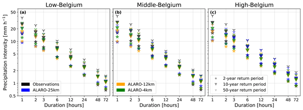
- Figure 6: “Intensity-Duration-Frequency (IDF) curves…”, but you do not show curves in this figure. Also mention that you use a log-log scale in the caption on both axes. Furthermore: “… stations observations or simulations…” --> “… station observations or simulations…”.
- Response: The figure shows markers rather than continuous curves, and no IDF relation is fitted or plotted. We have therefore replaced "IDF curves" with "IDF statistics" throughout the extreme-precipitation analysis. The Fig. 6 caption now describes the plotted elements as markers showing return levels versus duration on a log-log scale (both axes), and "Intensity-Duration-Frequency (IDF)" is retained only as the framework name at first mention. The typo "stations observations" is corrected to "station observations".
- Manuscript change: "IDF curves" → "IDF statistics" throughout the extreme-precipitation sections (Sects. 2.4, 3.2, 4.2); Fig. 6 caption revised (plot description clarified as markers, log-log scale on both axes stated, "stations observations" → "station observations").
- L248-L255: This part is somewhat hard to follow. Also please define R2here and notice that you do not show a fitted linear trend in the figures even though you discuss them in the text.
- Response: We have restructured this passage for clarity, separating the linear-fit procedure, the slope comparison, the R² comparison, and the return-period dependence. R² is now defined at first use as the coefficient of determination (the fraction of variance in the return levels explained by the linear fit). We also clarify that the fitted regression lines are not overlaid on Fig. 6; the slopes and R² values are presented in Fig. D3.
- Manuscript change: Sect. 3.2 paragraph rewritten: R² defined, explicit pointer that fits are quantified in Fig. D3 (L339-353).
- L259: “… was large” --> “… is large”.
- Response + Manuscript change: Updated as requested (L357).
- Figure 7: You have defined the whiskers, but also define the confidence interval that the boxes represent. Please also add (a), (b), etc. to the panels and use them in the caption and the text.
- Response: The caption now defines both elements: the box spans the interquartile range (25th–75th percentile) around the median, and the whiskers the 95% confidence interval (2.5th–97.5th percentile), both from the 10⁸-sample bootstrap. Panel labels (a)–(i), ordered row-wise (rows: regions Low-/Middle-/High-Belgium; columns: return periods 2, 10, 50 years), have been added to the figure and caption. The main text now references panels by letter where specific cells are discussed (Fig. 7a,d for sub-daily events in Low- and Middle-Belgium; Fig. 7g–i for multi-daily events in High-Belgium).
- Manuscript change: Fig. 7 caption revised (box + whisker definitions added, panel letters (a)–(i) added); figure regenerated with panel labels; in-text panel references added at two locations in the Sect. 3.2 discussion (L359, L361).
- L264: “…extremes increase…”, in intensity I suppose?
- Response + Manuscript change: Indeed, we have added “in intensity” to the sentence (L362).
- L270-L271: “Furthermore, the observational data set reveal a secondary peak in the early morning, which is absent in all simulations”. Do you have any idea why?
- Response: We investigated this and concluded the early-morning peak is most likely not robust: it does not appear in the peaks-over-threshold analysis of Van de Vyver et al. (2021) and has no established counterpart in the mid-latitude literature. Verifying it against the more recent observational networks is impractical, as extracting extreme-event timing is obstructed by heterogeneous time steps (1 min–1 h), differing formats, and missing values. As we do not consider it reliable, we have removed its discussion rather than interpret it as a physical signal.
- Manuscript change: Sect. 3.2: removed the two sentences discussing the secondary early-morning peak and the associated ALARO-25km nighttime-frequency remark.
- L281: “This difference in configuration might explain the clear distinction between these two sets of simulations” and L298: “This suggests that the use of SURFEX is responsible for the improved temperature bias”. This should be explored in more detail (see general comments). Also consider using the root-mean-square error as a metric.
- Response: With the ALARO-12km-noSFX experiment in place, the previously speculative attribution is demonstrated: the Discussion (Sect. 4.1) now states, on this basis, that the land-surface scheme (not the resolution increase) is responsible for the improved temperature bias and dominates the change in average precipitation. The referee's alternative, that the 25→12 km jump drives the change, is directly tested and shown to be secondary. The root-mean-square-error is addressed in an earlier comment.
- Manuscript change: Sect. 4.1; three attribution sentences rewritten to cite Sect. 3.3 (L407-409, L426-428, L432-434).
- L302: “These patters indicate that the inclusion of SURFEX exerts a greater influence on average precipitation than changes in spatial resolution”. Or it could be that the jump from 25 to 12 km resolution matters considerably, but it is hard to say without more analysis on the impact of SUFRFEX (see general comments).
- Response: This is the same confound raised in the previous comment and in our response on isolating the SURFEX effect, and is resolved by the same ALARO-12km-noSFX experiment.
- Manuscript change: We refer to the changes made under the previous comment.
- L304: “Our results for rainfall (Fig. 4) …”, but Fig. 4 shows the precipitation according to the caption, so it is not only rainfall I suppose?
- Response: Indeed, this was changed to precipitation, together with all other occurrences of the term rainfall, as explained in a previous comment.
- L305: “The annual bias from ALARO-25km is slightly larger than the bias over Middle Europe…”. Please quantify this by mentioning the biases from this study and the bias over Middle Europe.
- Response: We have quantified the comparison. ALARO-25km has an annual wet bias of 33.7 % over Belgium, ALARO-12km 15.3 %, and ALARO-4km 17.0 %. Giot et al. (2016) report an annual precipitation bias of approximately 20 % over Middle Europe for both their 50 and 12.5 km simulations. ALARO-25km is therefore markedly larger, while ALARO-12km and ALARO-4km are somewhat smaller. We revised the sentence accordingly, correcting the earlier "slight" characterisation.
- Manuscript change: In Sect. 4.1 added the three simulation biases and the ~20 % ME value; "slightly larger" → "markedly larger" (L436-439).
- L327: “ALARO-4m” --> “ALARO-4km”.
- Response + Manuscript change: Typo and related verb fixed (L460-461).
- L326-L328: For winter precipitation … than those in De Troch (2016)”. Can you explain why?
- Response: Winter precipitation over Belgium is predominantly stratiform, so the spurious afternoon peak in the ALARO-0 simulation of De Troch (2016) indicates convective triggering when little is expected. Its near-absence in ALARO-1 is consistent with reduced spurious wintertime triggering. This reflects the broader change from ALARO-0 to ALARO-1: it cannot be attributed to 3MT, common to both versions, and the available output does not allow the responsible physics to be isolated further.
- Manuscript change: Added one sentence in Sect. 4.1 linking the flatter winter cycle to reduced spurious convective triggering (L461-464).
- L329-L336: Refer to subfigures here.
- Response: Panel references added: wet-hour winter → Fig. 5d, wet-hour summer → Fig. 5c, and the all-hour/wet-hour summary → Fig. 5a/5b.
- Manuscript change: three panel references added in the Sect. 4.1 wet-hour discussion paragraph.
- L333-L334: However, for all simulations, the diurnal peak is later than the observational peak, which is in contrast with results from De Troch (2016)”. Can you explain this?
- Response: We can narrow the possibilities, though not pinpoint the cause. As noted in an earlier response, this difference stems from the change from ALARO-0 to ALARO-1 and cannot be attributed to 3MT, which both versions share. We can also exclude the land-surface scheme: the ALARO-12km-noSFX experiment shows that SURFEX changes the amplitude of the diurnal cycle but leaves the peak timing unchanged (Sect. 3.3, Fig. 9c). The remaining likely origin is the broader physics update from ALARO-0 to ALARO-1 (e.g. the ACRANEB2 radiation and TOUCANS turbulence schemes) and/or differences in experimental setup between the two studies. In particular, De Troch (2016) reinitialized daily, whereas ours are continuous; daily restarts repeatedly reset the soil and boundary-layer state and can plausibly alter the phase of the diurnal cycle. We cannot isolate this from the available output and flag it for future work.
- Manuscript change: Sect. 4.1 (L470-476): the statement was rescoped to the summer wet-hour peak, and the contrast with De Troch (2016) sharpened to specify that their ALARO-0 peak was too early. A sentence was added noting, on the basis of ALARO-12km-noSFX, that the peak-timing shift is not caused by SURFEX (Fig. 9c).
- L342-L345: Do you have an idea why this drizzle bias exists?
- Response: The drizzle bias — too-frequent, too-light precipitation — is a well-documented RCM deficiency, arising because parameterised convection triggers on weak instability and releases it gradually. This is borne out by the wet-hour decomposition (Table 2): relative to the Uccle observations, ALARO-25km has too many wet hours and too weak an intensity, both improving toward ALARO-4km. The improvement with resolution reflects sharper humidity and updraught fields that reduce the widespread simultaneous triggering of the coarser runs; the residual bias in ALARO-4km is consistent with 3MT still parameterising part of the convective spectrum in the grey zone. We present these as established mechanisms from the literature and have not isolated their contributions, as the required tendency terms are not stored.
- Manuscript change: Sect. 4.2: added the drizzle-bias mechanism, pointing to Table 2 (frequency vs. intensity decomposition); removed three redundant sentences restating the finding (L480-495).
- L352: No curves are plotted in Fig 6., but I understand what you mean.
- Response: As in our response to the earlier comment on Fig. 6, we have replaced "IDF curves" with "IDF statistics" throughout the extreme-precipitation analysis, so the terminology matches the plotted elements (markers showing return levels versus duration on a log-log scale, as clarified in the Fig. 6 caption).
- Manuscript change: "IDF curves" → "IDF statistics" at this line and throughout the extreme-precipitation sections (see the earlier Fig. 6 comment).
- L372-L373: “For longer durations (>24 hours), ALARO-25km tends to overestimate return levels, particularly for short return periods”. Can you refer to a figure here and can you elaborate more?
- Response: We have added a reference to Fig. 7 (relative error of return-level intensities by region, duration, and return period), which shows this directly: for durations >24 h, ALARO-25km overestimates return levels, most clearly at the 2-year return period (Fig. 7a–c).
- Manuscript change: In Sect. 4.2, added a reference to Fig. 7 at the multi-day/short-return statement (L534-535).
- L380-L382: “This behaviour … at high resolutions”. So why does this happen then?
- Response: This question prompted us to reconsider the paragraph. The original reasoning was flawed: we had assumed the scale-aware 3MT scheme should yield resolution-independent extreme-precipitation statistics, which is not correct. Scale-awareness only provides a smooth transition from parameterised to explicit convection as resolution increases; convection remains largely parameterised at coarse resolution and largely resolved at fine resolution, so differences between resolutions are in fact expected. What motivated the original paragraph was the perceived "step-wise" change from ALARO-12km to ALARO-4km, relative to the smaller change from ALARO-25km to ALARO-12km. We now offer two explanations. First, the 25 km to 12 km change may have been suppressed by the confounding drying effect of introducing SURFEX (Sect. 3.3). Second, the 12 km to 4 km step crosses the grey zone of convection, where a large shift in the partitioning between parameterised and resolved convection is expected. We have reframed the paragraph accordingly and left the isolation of these two effects to future work.
- Manuscript change: Sect. 4.2 paragraph reframed in terms of the reasoning above, replacing the earlier resolution-independence framing (L539-554). The final sentence of the abstract, which likewise alluded to resolution-independence, has been shortened to remove that claim (L14-17).
- L388-L390: The diurnal cycle … of this work”. Do you know why your work differs to the work of Van De Vyver er al. (2021)?
- Response: This difference reflects the same ALARO-0 to ALARO-1 contrast discussed in our responses to the comments on L326–328 and L333–334: the stronger resolution sensitivity of the diurnal cycle in ALARO-1 most plausibly stems from the broader physics update (e.g. ACRANEB2, TOUCANS), rather than from the scale-aware 3MT scheme, common to both. We cannot isolate the responsible change from the available output and have flagged it for future work.
- Manuscript change: A sentence was added following the Van de Vyver et al. (2021) comparison in Sect. 4.2 to attribute the stronger resolution sensitivity to the ALARO-0 to ALARO-1 physics update (L563-565).
- L405: You could mention that the introduction of SURFEX could be important as well, as it is suggested here that only resolution is relevant.
- Response: We agree. Following the ALARO-12km-noSFX experiment (Sect. 3.3), the conclusions now state that the improvement from ALARO-25km to the higher-resolution simulations is due not to resolution alone but substantially to SURFEX, which accounts for a large part of the reduction in temperature and precipitation biases. We have revised the average-climatology conclusion paragraph accordingly.
- Manuscript change: Added a sentence to the average-climatology conclusion paragraph attributing part of the improvement to SURFEX and pointing to Sect. 3.3 (L582-584).
- L409-L413: The scale aware scheme 3MT should be mentioned here or elsewhere in the conclusions, as it is an important finding of this study that the precipitation biases generally decrease with increased resolution despite 3MT.
- Response: We prefer to keep 3MT out of the conclusions, as it functions less as an object of study than as the feature enabling a clean multi-resolution setup. The added value of higher resolution is stated directly in the conclusions, while its relation to 3MT is developed in Sect. 4.2 (see previous comment).
- L453: Define F(x) here.
- Response + Manuscript change: We specified F(x) in the line introducing its mathematical form (L631).
References
- Ban, N., Schmidli, J., & Schär, C. (2014). Evaluation of the convection-resolving regional climate modeling approach in decade-long simulations. Journal of Geophysical Research: Atmospheres, 119(13), 7889–7907. https://doi.org/10.1002/2014JD021478
- Berthou, S., Kendon, E. J., Chan, S. C., Ban, N., Leutwyler, D., Schär, C., & Fosser, G. (2020). Pan-European climate at convection-permitting scale: A model intercomparison study. Climate Dynamics, 55(1), 35–59. https://doi.org/10.1007/s00382-018-4114-6
- Bertrand, C., Gonzalez Sotelino, L., & Journée, M. (2013). Quality control of 10-min air temperature data at RMI. Advances in Science and Research, 10(1), 1–5. https://doi.org/10.5194/asr-10-1-2013
- Bertrand, C., Ingels, R., & Journée, M. (2021). Homogenization and trends analysis of the Belgian historical precipitation time series. International Journal of Climatology, 41(11), 5277–5294. https://doi.org/10.1002/joc.7129
- Catry, B., Geleyn, J.-F., Bouyssel, F., Cedilnik, J., Broková, R., Derková, M., & Richard. (2008). A new sub-grid scale lift formulation in a mountain drag parameterisation scheme. Meteorologische Zeitschrift, 17(2), 193–208. https://doi.org/10.1127/0941-2948/2008/0272
- Clapp, R. B., & Hornberger, G. M. (1978). Empirical equations for some soil hydraulic properties. Water Resources Research, 14(4), 601–604. https://doi.org/10.1029/WR014i004p00601
- De Troch, R. (2016). The application of the ALARO-0 model for regional climate modeling in Belgium: Extreme precipitation and unfavorable conditions for the dispersion of air pollutants under present and future climate conditions [Dissertation, Ghent University]. http://hdl.handle.net/1854/LU-7247081
- Delvaux, C., Ingels, R., Vrábeĺ, V., Journée, M., & Bertrand, C. (2019). Quality control and homogenization of the Belgian historical temperature data. International Journal of Climatology, 39(1), 157–171. https://doi.org/10.1002/joc.5792
- Demarée, G. R. (2003). Le pluviographe centenaire du plateau d’Uccle: Son histoire, ses données et ses applications. La Houille Blanche, 89(4), 95–102. https://doi.org/10.1051/lhb/2003082
- Douville, H., Royer, J.-F., & Mahfouf, J.-F. (1995). A new snow parameterization for the Météo-France climate model. Climate Dynamics, 12(1), 21–35. https://doi.org/10.1007/BF00208760
- Ďurán, I. B., Geleyn, J.-F., & Váňa, F. (2014). A Compact Model for the Stability Dependency of TKE Production–Destruction–Conversion Terms Valid for the Whole Range of Richardson Numbers. Journal of the Atmospheric Sciences, 71(8), 3004–3026. https://doi.org/10.1175/JAS-D-13-0203.1
- Geleyn, J. ‐F., Mašek, J., Brožková, R., Kuma, P., Degrauwe, D., Hello, G., & Pristov, N. (2017). Single interval longwave radiation scheme based on the net exchanged rate decomposition with bracketing. Quarterly Journal of the Royal Meteorological Society, 143(704), 1313–1335. https://doi.org/10.1002/qj.3006
- Gerard, L., Piriou, J.-M., Brožková, R., Geleyn, J.-F., & Banciu, D. (2009). Cloud and Precipitation Parameterization in a Meso-Gamma-Scale Operational Weather Prediction Model. Monthly Weather Review, 137(11), 3960–3977. https://doi.org/10.1175/2009MWR2750.1
- Giot, O., Termonia, P., Degrauwe, D., De Troch, R., Caluwaerts, S., Smet, G., Berckmans, J., Deckmyn, A., De Cruz, L., De Meutter, P., Duerinckx, A., Gerard, L., Hamdi, R., Van Den Bergh, J., Van Ginderachter, M., & Van Schaeybroeck, B. (2016). Validation of the ALARO-0 model within the EURO-CORDEX framework. Geoscientific Model Development, 9(3), 1143–1152. https://doi.org/10.5194/gmd-9-1143-2016
- Journée, M., Ingels, R., & Bertrand, C. (2019). Overview and validation of observational gridded data products for Belgium.
- Lopez, P. (2002). Implementation and validation of a new prognostic large-scale cloud and precipitation scheme for climate and data-assimilation purposes. Quarterly Journal of the Royal Meteorological Society, 128(579), 229–257. https://doi.org/10.1256/00359000260498879
- Lucas-Picher, P., Argüeso, D., Brisson, E., Tramblay, Y., Berg, P., Lemonsu, A., Kotlarski, S., & Caillaud, C. (2021). Convection-permitting modeling with regional climate models: Latest developments and next steps. WIREs Climate Change, 12(6), e731. https://doi.org/10.1002/wcc.731
- Marquet, P., & Geleyn, J. (2013). On a general definition of the squared Brunt–Väisälä frequency associated with the specific moist entropy potential temperature. Quarterly Journal of the Royal Meteorological Society, 139(670), 85–100. https://doi.org/10.1002/qj.1957
- Mašek, J., Geleyn, J.-F., Brožková, R., Giot, O., Achom, H. O., & Kuma, P. (2016). Single interval shortwave radiation scheme with parameterized optical saturation and spectral overlaps. Quarterly Journal of the Royal Meteorological Society, 142(694), 304–326. https://doi.org/10.1002/qj.2653
- Prein, A. F., Langhans, W., Fosser, G., Ferrone, A., Ban, N., Goergen, K., Keller, M., Tölle, M., Gutjahr, O., Feser, F., Brisson, E., Kollet, S., Schmidli, J., van Lipzig, N. P. M., & Leung, R. (2015). A review on regional convection-permitting climate modeling: Demonstrations, prospects, and challenges. Reviews of Geophysics, 53(2), 323–361. https://doi.org/10.1002/2014RG000475
- Tabari, H., De Troch, R., Giot, O., Hamdi, R., Termonia, P., Saeed, S., Brisson, E., Van Lipzig, N., & Willems, P. (2016). Local impact analysis of climate change on precipitation extremes: Are high-resolution climate models needed for realistic simulations? Hydrology and Earth System Sciences, 20(9), 3843–3857. https://doi.org/10.5194/hess-20-3843-2016
- Termonia, P., Fischer, C., Bazile, E., Bouyssel, F., Brožková, R., Bénard, P., Bochenek, B., Degrauwe, D., Derková, M., El Khatib, R., Hamdi, R., Mašek, J., Pottier, P., Pristov, N., Seity, Y., Smolíková, P., Španiel, O., Tudor, M., Wang, Y., … Joly, A. (2018). The ALADIN System and its canonical model configurations AROME CY41T1 and ALARO CY40T1. Geoscientific Model Development, 11(1), 257–281. https://doi.org/10.5194/gmd-11-257-2018
- Van de Vyver, H., Van Schaeybroeck, B., De Troch, R., De Cruz, L., Hamdi, R., Villanueva-Birriel, C., Marbaix, P., van Ypersele, J.-P., Wouters, H., Vanden Broucke, S., van Lipzig, N. P. M., Doutreloup, S., Wyard, C., Scholzen, C., Fettweis, X., Caluwaerts, S., & Termonia, P. (2021). Evaluation Framework for Subdaily Rainfall Extremes Simulated by Regional Climate Models. Journal of Applied Meteorology and Climatology, 60(10), 1423–1442. https://doi.org/10.1175/JAMC-D-21-0004.1
-
AC1: 'Reply on RC1', Wout Dewettinck, 17 Jul 2026
-
RC2: 'Comment on egusphere-2025-2043', Anonymous Referee #2, 01 May 2026
Review of “Validation of the ALARO1-SFX (CY43T2) regional climate model over Belgium across different resolutions” (egusphere-2025-2043)
General comments
This study presents a multi-resolution validation of the ALARO1-SFX model over Belgium, with emphasis on temperature and precipitation biases, the diurnal cycle, and extreme precipitation statistics. The topic is relevant for GMD and the experimental design (multi-level dynamical downscaling) is sound. However, several important aspects need to be strengthened before the paper can be accepted as a full validation study.
- The validation relies primarily on station-based data (gridded from stations). Satellite products such as GPM (Global Precipitation Measurement) are not used. While satellite retrievals have uncertainties, they could provide valuable information on the spatial distribution of precipitation (including extremes and diurnal cycle) and help identify the origin of model biases.
- The authors aim to assess the added value of increasing resolution from the mesoscale to convection-permitting scales, partly to test the scale-aware 3MT scheme. However, the 12.5 km simulation is not truly in the “grey zone”(4-10 km) where both parameterised and explicit convection are relevant. To properly demonstrate the advantage of 3MT, a sensitivity experiment with deep convection fully turned off at 4 km (i.e., a purely explicit run) would be needed to isolate the contribution of the scale-aware scheme. Without such a comparison, the claimed added value of 3MT remains circumstantial.
- The study uses the hydrostatic dynamical core for all simulations, including the 4 km convection-permitting run. At this resolution, non-hydrostatic effects (e.g., strong convective updrafts) are often non-negligible. The authors should justify why the hydrostatic assumption is still valid at 4 km, or at least discuss the potential impact of this choice on the results, especially on hourly extreme precipitation and its diurnal cycle.
- The explanation for temperature biases (e.g., coastal vs. inland patterns, seasonal compensation) is rather speculative. The authors do not analyse temperature advection, surface albedo, cloud cover, or surface energy fluxes. For instance, the apparent anti-phase relationship between temperature and precipitation biases (Figs. 1D and 2D) suggests that cloud-radiation or soil-moisture feedbacks may be at play. A more process-based analysis (e.g., using radiation and turbulent flux outputs) is necessary to understand the sources of the temperature biases and why they change with resolution.
- The study focuses on IDF curves and return levels, which are interesting but somewhat difficult to interpret (Fig. 6). Conventional diagnostics such as precipitation frequency (wetday frequency), mean precipitation intensity, percentiles (e.g., 99.9th), and the spatial distribution of the diurnal peak are largely missing. These metrics could clearly demonstrate the common “too-light-too-frequent”bias at low resolution and would better illustrate the added value of the 4 km simulation and the scale-aware 3MT scheme.
Specific and technical comments
- L39-45 The authors mention problems when convection parameterisation is turned off in the grey zone. Please specify these problems more concretely (e.g., excessively strong or too-rare deep convection, biases in precipitation intensity and frequency, misrepresentation of the diurnal cycle). Moreover, a brief summary of existing scale-aware convection schemes and their typical behaviour would help contextualise the 3MT scheme. This paragraph might be better placed after line 56 and merged with lines 57-64.
- L190-194 Dividing Belgium into three regions based on elevation is reasonable. However, it would be helpful to show the observed mean annual precipitation for each region to verify that the regions indeed have distinct precipitation climates, as assumed.
- L212-221 The interpretation of temperature biases in terms of seasonal compensation and SST lag is interesting but speculative. To strengthen the analysis, please examine temperature advection, surface albedo, cloud cover (from the model output), and possibly surface energy fluxes. This would help to understand the cause of temperature biases.
- L222-228 The authors discuss annual and seasonal precipitation biases, but they do not separate precipitation frequency from intensity. The “wet bias” could arise from either too frequent events, too high intensity, or both. Analysing these two components separately (e.g., using maps or domain-averaged values) would better demonstrate the added value of higher resolution.
- L239-241 The statement that “ALARO-25km tends to produce too many light precipitation events” could be shown much more convincingly with simple maps of precipitation frequency and mean intensity. These would visually confirm the “raining too often with too little intensity” behaviour without resorting to the word “tends”. Similarly, the analysis of the diurnal cycle (Fig. 8) uses only station-aggregated data. The authors should consider using GPM data to examine the spatial distribution of the diurnal peak across Belgium.
- Fig. 6 The IDF plots are dense and difficult to read because each panel contains many markers for different return periods and durations. Consider separating return periods (e.g., different panels) and connecting points with lines. Alternatively, using precipitation percentiles (e.g., the 99.9th percentile of each duration) might provide a simpler and more direct comparison among the simulations.
- L270-271 The secondary morning peak in the observed diurnal cycle is very interesting. However, since the figure shows an ensemble over all stations, it may mask regional differences (some stations may have a morning peak, others only an afternoon peak). The authors are encouraged to use GPM or a high-resolution gridded product to map the spatial distribution of the diurnal peak timing. This could reveal whether the model’s failure to capture the morning peak is due to poor performance in specific areas.
- L298 The statement “This suggests that the use of SURFEX is responsible for the improved temperature bias” is too strong without process-based evidence. Please analyse temperature advection, surface albedo, cloud cover, and/or surface fluxes to support this attribution. Currently, it is not clear whether the improvement comes from SURFEX itself or from the higher resolution (or both).
- L339-340 “This implies that the precipitation frequency is overestimated.” This claim can be easily verified with a spatial map of precipitation frequency (e.g., number of wet hours per year or season). Please add such a figure to directly support the statement.
- L349-350 The statement that the later diurnal peak at lower resolutions “may be attributable to the scale-aware character of the 3MT scheme” is plausible, but the difference could also be caused by the land-surface scheme (ISBA vs. SURFEX) or by other aspects of the physics. A more cautious wording or a short sensitivity test (e.g., running ALARO-12km with ISBA) would help to isolate the cause.
Citation: https://doi.org/10.5194/egusphere-2025-2043-RC2 -
AC2: 'Reply on RC2', Wout Dewettinck, 17 Jul 2026
We thank the referee for the careful reading of our manuscript and for the constructive comments, which have helped us to improve the paper. Before addressing the individual comments, we summarise the most important changes made to the manuscript.
- New "Effect of SURFEX" section (Sect. 3.3). Responding to the referee’s call for a more process-based understanding of the temperature biases and firmer attribution of the SURFEX effect, we added a sensitivity experiment, ALARO-12km-noSFX. This experiment is identical to ALARO-12km but retains the ISBA land-surface scheme, which isolates the land-surface effect at a fixed 12.5 km. Together with a new surface energy-balance analysis (Figs. 9, 10, D4), it shows that the temperature difference between the ISBA and SURFEX configurations arises from a shift from latent to sensible heat flux at essentially unchanged net surface radiation, consistent with reduced soil moisture. As the other referee also requested it, it is the central revision of the manuscript.
- Precipitation frequency–intensity decomposition (Table 2). We decomposed the mean hourly precipitation into wet-hour frequency and intensity, quantifying the "too-light-too-frequent" bias directly. The wet-hour frequency falls from 17.2 % at 25 km to 14.8 % at 4 km (11.8 % observed) while the wet-hour intensity rises from 0.692 to 0.768 mm h⁻¹ (0.791 mm h⁻¹ observed). This more clearly demonstrates the added value of higher resolution.
- Hydrostatic core and grey-zone context. We added a justification for using the hydrostatic dynamical core at 4 km (Sect. 2.1.2) and expanded the introduction with a discussion of the grey zone of convection and scale-aware parameterisation schemes.
Line numbers in the 'Manuscript change' items refer to the marked-up (tracked-changes) manuscript.
General comments:
- The validation relies primarily on station-based data (gridded from stations). Satellite products such as GPM (Global Precipitation Measurement) are not used. While satellite retrievals have uncertainties, they could provide valuable information on the spatial distribution of precipitation (including extremes and diurnal cycle) and help identify the origin of model biases.
- Response: We chose not to incorporate satellite precipitation products. The Belgian rain-gauge network is dense and provides long, homogeneous records at daily (CLIMATE-GRID) and hourly (five networks, Table C1) resolution; the extreme-precipitation and AM-frequency analyses (Figs. 6–8) draw on this network directly. For a mid-latitude land domain the size of Belgium, this gauge basis is more accurate than satellite retrievals such as GPM, which carry non-negligible biases for light and sub-daily precipitation. Adopting a satellite product would add observational uncertainty rather than reduce it.
- The authors aim to assess the added value of increasing resolution from the mesoscale to convection-permitting scales, partly to test the scale-aware 3MT scheme. However, the 12.5 km simulation is not truly in the “grey zone”(4-10 km) where both parameterised and explicit convection are relevant. To properly demonstrate the advantage of 3MT, a sensitivity experiment with deep convection fully turned off at 4 km (i.e., a purely explicit run) would be needed to isolate the contribution of the scale-aware scheme. Without such a comparison, the claimed added value of 3MT remains circumstantial.
- Response: We agree that a 4 km run with deep convection switched off would be a natural way to isolate the contribution of the scale-aware 3MT scheme. However, we have opted not to include it, for two reasons.
- First, this is largely a matter of scope. This paper evaluates the ALARO1-SFX system as configured and used in climate applications, kept as close as possible to the operationally tuned model, which is well tuned for numerical weather prediction over Belgium. It is a model evaluation rather than a sensitivity study of the convection scheme. Isolating the contribution of 3MT by disabling deep convection at 4 km would amount to a separate sensitivity study of the convection parameterisation, beyond the evaluation objective here. We have already added one sensitivity experiment (ALARO-12km-noSFX, Sect. 3.3) to disentangle the SURFEX and resolution effects, and prefer to leave a further convection-scheme experiment to future work.
- Second, the requested experiment would be computationally demanding. Each simulation spans 32 years, and a 4 km convection-off integration of comparable length would carry a considerable cost, on top of the ALARO-12km-noSFX experiment added during this revision.
- Response: We agree that a 4 km run with deep convection switched off would be a natural way to isolate the contribution of the scale-aware 3MT scheme. However, we have opted not to include it, for two reasons.
- The study uses the hydrostatic dynamical core for all simulations, including the 4 km convection-permitting run. At this resolution, non-hydrostatic effects (e.g., strong convective updrafts) are often non-negligible. The authors should justify why the hydrostatic assumption is still valid at 4 km, or at least discuss the potential impact of this choice on the results, especially on hourly extreme precipitation and its diurnal cycle.
- Response: We agree this warrants explicit justification. Our choice of the hydrostatic core at 4 km is deliberate and rests on two considerations.
- First, Van Ginderachter et al. (2020) ran the ALARO model at 4 km over a tropical domain of intense deep convection in both hydrostatic and non-hydrostatic configurations. The hydrostatic version performed better, because the ALARO physics package, including the 3MT deep-convection scheme, was developed and tuned with the hydrostatic core. Their subsequent ensemble tests with the two cores led to identical conclusions. This indicates that, for the precipitation and diurnal-cycle diagnostics here, the hydrostatic choice does not compromise the results at 4 km, and staying with the operationally tuned configuration is preferable to an untuned non-hydrostatic setup.
- Second, this matches operational practice: the ALARO model is run for NWP at ~4 km with the hydrostatic core, and remaining close to the operational configuration, which is well tuned for extreme precipitation over Belgium and Europe, is a deliberate design choice of this evaluation. Using the same hydrostatic core across all three resolutions (25, 12.5, 4 km) also lets the resolution dependence be studied without confounding it with a change of dynamical core.
- Manuscript change: Added a short justification of the hydrostatic choice to Sect. 2.1.2 (L174-180).
- Response: We agree this warrants explicit justification. Our choice of the hydrostatic core at 4 km is deliberate and rests on two considerations.
- The explanation for temperature biases (e.g., coastal vs. inland patterns, seasonal compensation) is rather speculative. The authors do not analyse temperature advection, surface albedo, cloud cover, or surface energy fluxes. For instance, the apparent anti-phase relationship between temperature and precipitation biases (Figs. 1D and 2D) suggests that cloud-radiation or soil-moisture feedbacks may be at play. A more process-based analysis (e.g., using radiation and turbulent flux outputs) is necessary to understand the sources of the temperature biases and why they change with resolution.
- Response: The referee requests three analyses (surface energy fluxes, cloud cover/albedo, and temperature advection) plus the anti-phase temperature–precipitation relationship. We address each below.
- Surface energy fluxes. We have added a process-based surface energy-balance analysis (Sect. 3.3, Figs. 10 and D4), in the context of isolating the SURFEX land-surface scheme. The temperature difference between the ISBA and SURFEX configurations arises from a shift in the partitioning of the latent and sensible heat fluxes (reduced latent and increased sensible heat, strongest in summer) at essentially unchanged net surface radiation. This identifies surface-flux partitioning, consistent with reduced soil moisture, as the source of the scheme-dependent temperature bias, supporting the soil-moisture-feedback hypothesis the referee raises.
- Cloud cover / albedo. Across all configurations, the net surface radiation is essentially unchanged (Fig. D4), so the available surface energy is the same and the flux differences are consistent with being driven by the surface state; a cloud- or radiation-driven explanation is not required (Sect. 3.3). We therefore do not present a separate cloud-cover analysis for this contrast.
- Temperature advection. We cannot analyse temperature advection, as the advective tendency terms are not stored in the model output and cannot be reconstructed a posteriori.
- Anti-phase temperature–precipitation relationship (Figs. D1, D2). This is consistent with the soil-moisture mechanism in Sect. 3.3: reduced soil moisture in the SURFEX configuration simultaneously suppresses evaporative cooling (warming) and reduces precipitation. The coastal temperature patterns and their seasonal compensation, also noted by the referee, are addressed separately through the SST-lag and coastal tile-weighting mechanisms (Sect. 3.1, in response to Referee 1).
- Manuscript change: New Sect. 3.3 (Figs. 9, 10, D4); coastal tile-weighting sentence in Sect. 3.1 (L294-296).
- Response: The referee requests three analyses (surface energy fluxes, cloud cover/albedo, and temperature advection) plus the anti-phase temperature–precipitation relationship. We address each below.
- The study focuses on IDF curves and return levels, which are interesting but somewhat difficult to interpret (Fig. 6). Conventional diagnostics such as precipitation frequency (wetday frequency), mean precipitation intensity, percentiles (e.g., 99.9th), and the spatial distribution of the diurnal peak are largely missing. These metrics could clearly demonstrate the common “too-light-too-frequent” bias at low resolution and would better illustrate the added value of the 4 km simulation and the scale-aware 3MT scheme.
- Response: IDF curves and return levels, although less intuitive than mean-state diagnostics, are of considerable practical relevance. Return-level maps, including their evolution under climate change, are a primary input for hydrological design and flood-risk assessment. We further address each of the four suggested diagnostics.
- Precipitation frequency. New Table 2 reports the wet-hour frequency for the observations and each simulation, at hourly resolution (the relevant scale for the convective, sub-daily extremes that are the focus of this study). It directly shows the "too-frequent" component of the bias and its monotonic reduction with resolution (17.2 % at 25 km → 14.8 % at 4 km vs. 11.8 % observed).
- Mean precipitation intensity. This is already the study's primary precipitation diagnostic: the mean (relative) precipitation bias is reported annually, seasonally, and monthly (Figs. 4, D2, 3), and the wet-hour mean intensity is now additionally reported in Table 2, showing the complementary "too-light" component (0.692 mm h⁻¹ at 25 km → 0.768 mm h⁻¹ at 4 km vs. 0.791 mm h⁻¹ observed). Together with the frequency, this quantifies the "too-light-too-frequent" bias the referee refers to.
- High percentiles (e.g., 99.9th). While high hourly percentiles are an interesting and interpretable diagnostic, we keep the focus on the far upper tail of the precipitation distribution, characterised through extreme-value statistics (annual maxima and GEV return levels). This reflects the study's scope, i.e. to assess the added value of increasing resolution. As this is mainly expected for convective processes, we focus on sub-daily convective extremes. They also allow direct comparison with earlier work over Belgium (De Troch, 2016; Tabari et al., 2016; Van de Vyver et al., 2021). The added value of the 4 km simulation at the extreme tail is demonstrated on this basis (Sect. 3.2). We therefore prefer not to introduce the percentiles as an additional, differently-defined diagnostic.
- Spatial distribution of the diurnal peak. For a country as small as Belgium, a spatial map of the diurnal cycle of extreme hourly precipitation would carry little information and be very noisy. Most extreme hourly precipitation over Belgium originates from a limited number of passing convective systems (MCSs, frontal lines) that affect essentially the whole country within a single synoptic setting. This produces strong spatial and temporal coherence, but correspondingly few statistically independent samples per grid point, so a per-grid point diurnal map would not yield a robust or interpretable added-value signal. We therefore characterise the diurnal peak at the domain level (Fig. 8) rather than spatially.
- Manuscript change: Table 2 (wet-hour decomposition) added in Sect. 3.1, including supporting text in Sect. 3.1 and Sect. 4.2.
- Response: IDF curves and return levels, although less intuitive than mean-state diagnostics, are of considerable practical relevance. Return-level maps, including their evolution under climate change, are a primary input for hydrological design and flood-risk assessment. We further address each of the four suggested diagnostics.
Specific and technical comments:
- L39-45 The authors mention problems when convection parameterisation is turned off in the grey zone. Please specify these problems more concretely (e.g., excessively strong or too-rare deep convection, biases in precipitation intensity and frequency, misrepresentation of the diurnal cycle). Moreover, a brief summary of existing scale-aware convection schemes and their typical behaviour would help contextualise the 3MT scheme. This paragraph might be better placed after line 56 and merged with lines 57-64.
- Response: We have expanded the paragraph to specify the concrete problems arising in the grey zone and added a brief overview of the main approaches to scale-aware convective parameterisation, which contextualises 3MT. On placement, we have retained the paragraph in its original position: it describes the general setting (convection-permitting models, the grey zone, and scale-aware schemes as a class) whereas the subsequent paragraph bridges this to the present study by motivating ALARO1-SFX with 3MT specifically. Merging them would blur this deliberate progression from general context to study-specific motivation.
- Manuscript change: Expanded paragraph discussing the grey zone of convection (L44-48) and scale-aware parameterisation schemes (L51-54).
- L190-194 Dividing Belgium into three regions based on elevation is reasonable. However, it would be helpful to show the observed mean annual precipitation for each region to verify that the regions indeed have distinct precipitation climates, as assumed.
- Response: We have computed the observed mean annual precipitation for each region over 1992–2022: 838 mm (Low), 818 mm (Middle), and 1037 mm (High-Belgium), based on the CLIMATE-GRID dataset. The resulting figure is added as a supplement to this response. High-Belgium is clearly distinct, whereas Low- and Middle-Belgium are very similar. Nevertheless, the three-region delineation follows a standard, physically-motivated physiographic subdivision of Belgium based on elevation, consistent with the subdivision in the RMI Climate Atlas (https://www.meteo.be/nl/klimaat/klimaat-van-belgie/klimaatatlas/klimaatkaarten/neerslag/neerslaghoeveelheid/jaarlijks, unfortunately only available in Dutch and French). The Climate Atlas notes that annual precipitation normals are relatively uniform across Low- and Middle-Belgium, whereas the range is large in High-Belgium, consistent with our finding.
- L212-221 The interpretation of temperature biases in terms of seasonal compensation and SST lag is interesting but speculative. To strengthen the analysis, please examine temperature advection, surface albedo, cloud cover (from the model output), and possibly surface energy fluxes. This would help to understand the cause of temperature biases.
- Response: We have added surface energy-flux and net-radiation analyses (Sect. 3.3, Figs. 10, D4), which show the resolution-/scheme-dependent temperature differences arise from surface flux partitioning at unchanged net radiation, ruling out a cloud- or radiation-driven explanation. We do not include a temperature-advection analysis: the advective tendency terms are not stored in the model output, so this cannot be computed a posteriori. Surface albedo enters through the net-radiation diagnostic, which is unchanged across configurations.
- SURFEX warms the domain fairly uniformly except over urban areas (Fig. 9). Coastal cells, whose near-surface temperature is dominated by the sea tile, are among the least affected. The coastal bias is therefore governed mainly by the SST-lag and tile-weighting mechanisms discussed in Sect. 3.1 (in response to Referee 1), not by the land-surface scheme.
- Manuscript change: New Sect. 3.3 discussing the surface energy balance (Figs. 9, 10, D4); coastal-bias interpretation sentence added in Sect. 3.1.
- Response: We have added surface energy-flux and net-radiation analyses (Sect. 3.3, Figs. 10, D4), which show the resolution-/scheme-dependent temperature differences arise from surface flux partitioning at unchanged net radiation, ruling out a cloud- or radiation-driven explanation. We do not include a temperature-advection analysis: the advective tendency terms are not stored in the model output, so this cannot be computed a posteriori. Surface albedo enters through the net-radiation diagnostic, which is unchanged across configurations.
- L222-228 The authors discuss annual and seasonal precipitation biases, but they do not separate precipitation frequency from intensity. The “wet bias” could arise from either too frequent events, too high intensity, or both. Analysing these two components separately (e.g., using maps or domain-averaged values) would better demonstrate the added value of higher resolution.
- Response: Separating frequency from intensity clarifies the origin of the wet bias. We have added a decomposition of the mean hourly precipitation at Uccle into wet-hour frequency and intensity contributions (new Table 2), reporting the wet-hour frequency and mean wet-hour intensity for the observations and each simulation. The decomposition shows that the wet bias is driven by an overestimated wet-hour frequency (17.2 % at 25 km vs. 11.8 % observed) combined with an underestimated wet-hour intensity (0.692 vs. 0.791 mm h⁻¹), not by excessive intensity. Increasing resolution reduces the frequency bias and raises the wet-hour intensity, quantifying the added value of higher resolution. We chose the Uccle station rather than spatial maps because the sub-daily analysis is anchored to the hourly station data (Fig. 5). The station-based table gives the requested frequency–intensity separation on the same footing as the existing diurnal-cycle figure.
- Manuscript change: New Table 2 (wet-hour decomposition) in Sect. 3.1 with supporting text; Discussion Sect. 4.1 updated to cite the table.
- L239-241 The statement that “ALARO-25km tends to produce too many light precipitation events” could be shown much more convincingly with simple maps of precipitation frequency and mean intensity. These would visually confirm the “raining too often with too little intensity” behaviour without resorting to the word “tends”. Similarly, the analysis of the diurnal cycle (Fig. 8) uses only station-aggregated data. The authors should consider using GPM data to examine the spatial distribution of the diurnal peak across Belgium.
- Response: The comment raises two separate points, which we address in turn.
- Frequency/intensity of the general diurnal cycle. We have removed the hedged wording. The "raining too often with too little intensity" behaviour is now shown quantitatively in Table 2, which reports the wet-hour frequency and mean wet-hour intensity for the observations and each simulation (see our response to the related comment on conventional diagnostics). Both components, and their monotonic improvement with resolution, are now stated as demonstrated results rather than a tendency: the sentences in Sect. 3.1 (Fig. 5 paragraph) and Sect. 4.1 have been reworded accordingly, with "tends to" removed. We chose a decomposition table rather than frequency/intensity maps because the diagnostic of interest is the wet-hour statistics of the Uccle record, for which a table is more precise and comparable across simulations than a pair of spatial maps.
- Spatial distribution of the diurnal peak of extremes (Fig. 8). This is the diurnal cycle of annual-maximum hourly precipitation, which is distinct from the general diurnal cycle above. As explained in our response on the requested conventional diagnostics, a spatial map of the diurnal peak is not informative for a domain the size of Belgium: extreme hourly precipitation originates from a limited number of passing convective systems affecting essentially the whole country within one synoptic setting, producing strong spatial coherence but very few statistically independent samples per grid point. A per-grid point map would therefore be noisy and uninterpretable. GPM is not incorporated in this study, for the reasons given in our response on satellite data.
- Manuscript change: Rewritten paragraph in Sect. 3.1 to cite Table 2 (L287-295).
- Response: The comment raises two separate points, which we address in turn.
- 6 The IDF plots are dense and difficult to read because each panel contains many markers for different return periods and durations. Consider separating return periods (e.g., different panels) and connecting points with lines. Alternatively, using precipitation percentiles (e.g., the 99.9th percentile of each duration) might provide a simpler and more direct comparison among the simulations.
- Response: We agree the IDF plots are dense, but this presentation is necessary to give the complete picture: return-level behaviour across resolutions, durations, and return periods is best conveyed in a single figure. Spreading this across several panels would fragment a comparison that is most informative when shown as a whole. For a more detailed view, Fig. 7 already provides separate panels per region and return period. To address the referee's concern we have reduced clutter: redundant text removed, the legend spread across panels, and the markers enlarged for On precipitation percentiles, we refer to our response on conventional diagnostics above.
- Manuscript change: Figure 6 has been redrawn.
- L270-271 The secondary morning peak in the observed diurnal cycle is very interesting. However, since the figure shows an ensemble over all stations, it may mask regional differences (some stations may have a morning peak, others only an afternoon peak). The authors are encouraged to use GPM or a high-resolution gridded product to map the spatial distribution of the diurnal peak timing. This could reveal whether the model’s failure to capture the morning peak is due to poor performance in specific areas.
- Response: An aggregated cycle could in principle mask regional contrasts, but for this domain a spatially resolved map of the diurnal peak timing would not be robust or interpretable, for two related reasons. First, Belgium is small, and its extreme hourly precipitation is dominated by a limited number of passing convective systems (MCSs, frontal lines) that affect essentially the whole country within a single synoptic setting. This produces strong spatial and temporal coherence, so neighbouring locations largely share the same signal rather than exhibiting independent regional cycles. Second, and consequently, there are very few statistically independent samples per grid point: splitting the already-limited annual-maximum sample across locations leaves too little data to estimate peak timing reliably, and the resulting map would be dominated by sampling noise. This holds regardless of the observational source: GPM would not resolve it and would introduce its own retrieval and sampling biases. We also no longer interpret the secondary morning peak as a physical feature (see our response to the Referee 1 comment on L270–271).
- Manuscript change: The interpretation of the secondary morning peak has been removed from Sect. 3.2 (L368).
- L298 The statement “This suggests that the use of SURFEX is responsible for the improved temperature bias” is too strong without process-based evidence. Please analyse temperature advection, surface albedo, cloud cover, and/or surface fluxes to support this attribution. Currently, it is not clear whether the improvement comes from SURFEX itself or from the higher resolution (or both).
- Response: We address both halves. (i) Attribution: the ALARO-12km-noSFX experiment (Sect. 3.3, Fig. 9) isolates SURFEX from resolution and shows the improvement is predominantly due to SURFEX. (ii) Process evidence: the surface energy-balance analysis (Figs. 10, D4) demonstrates the mechanism: a shift from latent to sensible heating at essentially unchanged net radiation, consistent with reduced soil moisture. The claim is therefore now supported by both a controlled experiment and a process chain.
- Manuscript change: New Sect. 3.3; Discussion attribution sentences strengthened (L407-408, L426-428, L432-434, L501-503).
- L339-340 “This implies that the precipitation frequency is overestimated.” This claim can be easily verified with a spatial map of precipitation frequency (e.g., number of wet hours per year or season). Please add such a figure to directly support the statement.
- Response: The claim is now supported directly by new Table 2, which reports the wet-hour frequency for the observations and each simulation. All simulations overestimate the wet-hour frequency relative to the observed 11.8 %, most strongly at 25 km (17.2 %), decreasing with resolution to 15.0 % (12 km) and 14.8 % (4 km). We have accordingly reworded the Discussion from "this implies that the precipitation frequency is overestimated" to cite the quantified frequency in Table 2. We provide a station-based decomposition rather than a spatial wet-hour-frequency map to keep the frequency and intensity components on the same footing, tied to the hourly station record underlying the diurnal analysis.
- Manuscript change: Sect. 4.1 sentence reworded from an inference to a table-grounded statement citing Table 2 (L441-442).
- L349-350 The statement that the later diurnal peak at lower resolutions “may be attributable to the scale-aware character of the 3MT scheme” is plausible, but the difference could also be caused by the land-surface scheme (ISBA vs. SURFEX) or by other aspects of the physics. A more cautious wording or a short sensitivity test (e.g., running ALARO-12km with ISBA) would help to isolate the cause.
- Response: We have performed exactly the sensitivity test proposed. The ALARO-12km-noSFX experiment (12.5 km with ISBA, otherwise identical to ALARO-12km) isolates the land-surface contribution to the diurnal cycle. As shown in the new panel Fig. 9c, the two configurations share the same afternoon peak at 16–17 UTC; introducing SURFEX reduces the amplitude of the diurnal cycle but leaves the timing and shape of the peak unchanged. The land-surface scheme therefore does not drive the peak timing. We have accordingly replaced the assertion that the shift "may be attributable to the scale-aware character of the 3MT scheme" with a bounded attribution. Having ruled out the land-surface scheme, we attribute the timing to the convection scheme and identify the likely mechanism: conventional CAPE-closure mass-flux schemes remove instability almost as soon as surface heating generates it, peaking near local noon (Bechtold et al., 2004; Guichard et al., 2004), whereas the prognostic closure of 3MT retains memory of the updraught mesh fraction and velocity between time steps and releases instability gradually, shifting the peak to the afternoon. We present this as a plausible rather than demonstrated mechanism, and state explicitly that a full attribution would require dedicated sensitivity experiments, left to future work.
- Manuscript change: New panel Fig. 9c (diurnal cycle of precipitation, ALARO-12km vs. ALARO-12km-noSFX) and supporting sentence in Sect. 3.3 (L375-380). In Sect. 4.2, the wording was changed from asserting 3MT as the cause to a bounded attribution: the land-surface scheme is excluded on the basis of the isolation experiment, the prognostic-closure mechanism is offered as the likely explanation with supporting references, and the residual uncertainty is acknowledged explicitly (L546-554).
References
- Bechtold, P., Chaboureau, J.-P., Beljaars, A., Betts, A. K., Köhler, M., Miller, M., & Redelsperger, J.-L. (2004). The simulation of the diurnal cycle of convective precipitation over land in a global model. Quarterly Journal of the Royal Meteorological Society, 130(604), 3119–3137. https://doi.org/10.1256/qj.03.103
- De Troch, R. (2016). The application of the ALARO-0 model for regional climate modeling in Belgium: Extreme precipitation and unfavorable conditions for the dispersion of air pollutants under present and future climate conditions [Dissertation, Ghent University]. http://hdl.handle.net/1854/LU-7247081
- Guichard, F., Petch, J. C., Redelsperger, J.-L., Bechtold, P., Chaboureau, J.-P., Cheinet, S., Grabowski, W., Grenier, H., Jones, C. G., Köhler, M., Piriou, J.-M., Tailleux, R., & Tomasini, M. (2004). Modelling the diurnal cycle of deep precipitating convection over land with cloud-resolving models and single-column models. Quarterly Journal of the Royal Meteorological Society, 130(604), 3139–3172. https://doi.org/10.1256/qj.03.145
- Tabari, H., De Troch, R., Giot, O., Hamdi, R., Termonia, P., Saeed, S., Brisson, E., Van Lipzig, N., & Willems, P. (2016). Local impact analysis of climate change on precipitation extremes: Are high-resolution climate models needed for realistic simulations? Hydrology and Earth System Sciences, 20(9), 3843–3857. https://doi.org/10.5194/hess-20-3843-2016
- Van de Vyver, H., Van Schaeybroeck, B., De Troch, R., De Cruz, L., Hamdi, R., Villanueva-Birriel, C., Marbaix, P., van Ypersele, J.-P., Wouters, H., Vanden Broucke, S., van Lipzig, N. P. M., Doutreloup, S., Wyard, C., Scholzen, C., Fettweis, X., Caluwaerts, S., & Termonia, P. (2021). Evaluation Framework for Subdaily Rainfall Extremes Simulated by Regional Climate Models. Journal of Applied Meteorology and Climatology, 60(10), 1423–1442. https://doi.org/10.1175/JAMC-D-21-0004.1
- Van Ginderachter, M., Degrauwe, D., Vannitsem, S., & Termonia, P. (2020). Simulating model uncertainty of subgrid-scale processes by sampling model errors at convective scales. Nonlinear Processes in Geophysics, 27(2), 187–207. https://doi.org/10.5194/npg-27-187-2020
Peer review completion


Interactive discussion
Status: closed
-
RC1: 'Comment on egusphere-2025-2043', Anonymous Referee #1, 24 Apr 2026
This study presents an evaluation of the ALARO-1 model coupled to SURFEX on several resolutions for Belgium, with a focus on temperature and in particular precipitation. The authors show that higher resolutions improve modelled precipitation considerably despite the presence of a scale-aware convection scheme. The manuscript is generally well written and fits the scope of the journal, but more interpretation and evaluation of several variables have to be explored before it can be presented as a full evaluation paper. The following comments should help with solving the remaining issues before publication, with e.g. L1 referring to line 1.
General comments:
- In the manuscript it is described that SURFEX is introduced for the ALARO-12km and ALARO-4km simulations, while ISBA is used for ALARO-25km. SURFEX, however, is barely introduced and the chosen SURFEX settings are not explained. SURFEX has a multitude of options and parameterizations to choose from, many of them can significantly impact your results, especially temperature. To understand the biases in e.g. Figure 2 and whether they are caused by changing the resolution or by using SURFEX, it is crucial that SURFEX is properly introduced. More specifically I have several questions: how many soil layers are used, do you use ISBA-DIF, how many patches do you use for the nature tile, what do you use for runoff, root distributions, snow etc., and what do you use to calculate fluxes over water (ECUME or ECUME6 maybe)? Especially the number of soil layers can greatly impact modelled turbulence and near-surface temperature during dry months in spring or summer. See also some specific comments.
- The authors have compared their results extensively with previous work, but the manuscript could benefit from more interpretation in general of the results shown in this work, especially in the discussion section. Some specific comments are related to this.
- The manuscript is presented as an evaluation of ALARO-1, but more processes have to be studied to identify the strengths and weaknesses of the model before it can be presented as such. Analysis of the energy balance components (downward and upward shortwave and longwave radiative fluxes, sensible and latent heat fluxes) will provide valuable information about how well several aspects of the climate system are modelled and can be compared to in-situ observations. It could reveal for example problems during clear-sky conditions or cloudy conditions, to the albedo or turbulence, or a too dry soil during summer. It is thus imperative to understand why the temperature biases presented in Fig. 2, Fig. 3 and Fig. D1 occur and why they change with resolution. Adding a section about surface fluxes is thus desirable.
- Similar as last comment, as a new surface scheme is introduced, a short section about its impact on the model should be considered. If possible, running ALARO1-25km with SURFEX could reveal much of the impact of SURFEX when comparing with ALARO1-25 km that uses only ISBA. Processes like available soil moisture and runoff and its feedback on precipitation can be explored.
- The terms ‘validation’ and ‘evaluation’ are both used in the manuscript, but evaluation is the more suitable term for this study. I would recommend to use ‘evaluation’ consistently in the manuscript, including in the title.
- Showing statistical significance on the bias maps (Fig. 2, 4, D1, D2) could help improve interpretation of the results.
Specific and technical comments
- L13: Consider rephrasing: “Furthermore, the study provides experimental evidence…”
- L46: “… associated with the low-resolution parameterization of deep convection” --> “associated with the parameterization of deep convection used in lower resolution models”, or something similar.
- L57-L59: Can you be more specific what uncertainties you refer to?
- L58: “… uncertainties in the short term”, can you define ‘short term’ here?
- L65-L66 and elsewhere in the text: Make sure to define the abbreviations first before using the abbreviations, such as ALARO and ISBA, or ARPEGE on L112 and a few other lines.
- L66: But ISBA is also part of SURFEX, can you be more specific what will be replaced or introduced by SURFEX?
- L78-L81: Can you define here what you will evaluate in this study?
- Merge L84-L88 with L65-L71 as this should be mentioned earlier.
- L89: “… we evaluated long-term …” --> “… we evaluate long-term …”, and L93: “In contrast, this study utilized … ” --> “In contrast, this study utilizes … ”.
- L95: What do you mean with: “This new version marked a step-wise change compared to the original ALARO-0”?
- L111: Can you be more specific what parts of the IFS and of ARPEGE are left in ALARO?
- 2.1.1: Can you explain in more detail SURFEX (see general comments), but also what kind of radiative, turbulence and cloud schemes are used?
- L125: Please specify what variables are forced by ERA5 at the boundaries.
- L128-L129: Can you explain why you nest the 4 km run in the 12.5 km run and the 12.5 in the 25 km run; why do you not force all runs directly with ERA5?
- L137 and elsewhere: Readability would improve if you would refer to the panels of the figures by e.g., Fig. 1a.
- L146-L147: It makes it difficult to interpret whether the changes between the 12.5 and 25 km runs are caused by introduction of SURFEX or the resolution. Running on 25 km with SURFEX could help with this. Also more information about the chosen SURFEX is necessary (see general comments).
- L149: Please add a reference to the CLIMATE-GRID data set.
- L153-L154: Is precipitation measured the same way for all data sets? If not, consider adding this in Table C1.
- L159: “Rainfall data from all…”, earlier you mention that the observations are precipitation, but now you mention rainfall. So are these stations only measuring rainfall then or also snow?
- L173-L174: Please add a reference here.
- In Sect. 2.3 – 2.4, consider using the present tense.
- L183: Define that T-year and d-hourly as the return period and duration here.
- L196: Can you explain here why you want to use IDF curves?
- L204-L205: “Near the coast, all simulations exhibit a small warm bias”. Do you know why?
- Figure 2 and all other figures: Can you add over what time period these biases are calculated and use (a), (b), etc. for the panels and use (a), (b), etc. in the caption and in the text.
- L209-L215: This could be related to a different representation of the soil layers in SURFEX, but it is hard to say without more information about the SURFEX settings. SURFEX with ISBA-DIF has the tendency to dry out rather quickly in summer, raising the sensible heat flux and reducing the latent heat flux and consequently increasing the near-surface temperature, especially during dry years.
- L218: “The minimal bias” --> “The largest negative bias”.
- L219-L221: Just a thought, but could this be caused by accidentally using water grid points as well in the interpolation near the coast?
- L222-L223: “… and seasons (Fig. D2). A notable exception is the dry bias in summer (July and August)…” --> “… and seasons (Fig. D2), except for summer (July and August)…”
- L226: “ALARO-4km preforms best when evaluating the seasons separately”. Consider using the root-mean-square-error (RMSE) to quantify this.
- L233-L241: Please mention the subfigures here where you refer to, which would improve readability.
- Figure 6: “Intensity-Duration-Frequency (IDF) curves…”, but you do not show curves in this figure. Also mention that you use a log-log scale in the caption on both axes. Furthermore: “… stations observations or simulations…” --> “… station observations or simulations…”.
- L248-L255: This part is somewhat hard to follow. Also please define R2 here and notice that you do not show a fitted linear trend in the figures even though you discuss them in the text.
- L259: “… was large” --> “… is large”.
- Figure 7: You have defined the whiskers, but also define the confidence interval that the boxes represent. Please also add (a), (b), etc. to the panels and use them in the caption and the text.
- L264: “…extremes increase…”, in intensity I suppose?
- L270-L271: “Furthermore, the observational data set reveal a secondary peak in the early morning, which is absent in all simulations”. Do you have any idea why?
- L281: “This difference in configuration might explain the clear distinction between these two sets of simulations” and L298: “This suggests that the use of SURFEX is responsible for the improved temperature bias”. This should be explored in more detail (see general comments). Also consider using the root-mean-square error as a metric.
- L302: “These patters indicate that the inclusion of SURFEX exerts a greater influence on average precipitation than changes in spatial resolution”. Or it could be that the jump from 25 to 12 km resolution matters considerably, but it is hard to say without more analysis on the impact of SUFRFEX (see general comments).
- L304: “Our results for rainfall (Fig. 4) …”, but Fig. 4 shows the precipitation according to the caption, so it is not only rainfall I suppose?
- L305: “The annual bias from ALARO-25km is slightly larger than the bias over Middle Europe…”. Please quantify this by mentioning the biases from this study and the bias over Middle Europe.
- L327: “ALARO-4m” --> “ALARO-4km”.
- L326-L328: For winter precipitation … than those in De Troch (2016)”. Can you explain why?
- L329-L336: Refer to subfigures here.
- L333-L334: However, for all simulations, the diurnal peak is later than the observational peak, which is in contrast with results from De Troch (2016)”. Can you explain this?
- L342-L345: Do you have an idea why this drizzle bias exists?
- L352: No curves are plotted in Fig 6., but I understand what you mean.
- L372-L373: “For longer durations (>24 hours), ALARO-25km tends to overestimate return levels, particularly for short return periods”. Can you refer to a figure here and can you elaborate more?
- L380-L382: “This behaviour … at high resolutions”. So why does this happen then?
- L388-L390: The diurnal cycle … of this work”. Do you know why your work differs to the work of Van De Vyver er al. (2021)?
- L405: You could mention that the introduction of SURFEX could be important as well, as it is suggested here that only resolution is relevant.
- L409-L413: The scale aware scheme 3MT should be mentioned here or elsewhere in the conclusions, as it is an important finding of this study that the precipitation biases generally decrease with increased resolution despite 3MT.
- L453: Define F(x) here.
Citation: https://doi.org/10.5194/egusphere-2025-2043-RC1 -
AC1: 'Reply on RC1', Wout Dewettinck, 17 Jul 2026
We thank the referee for the careful reading of our manuscript and for the constructive comments, which have helped us to improve the paper. Before addressing the individual comments, we summarise the most important changes made to the manuscript.
- New "Effect of SURFEX" section (Sect. 3.3). The largest addition is a sensitivity experiment, ALARO-12km-noSFX, which is identical to ALARO-12km but retains the ISBA land-surface scheme. This experiment was run over the full 32-year period (1991–2022). Holding resolution fixed at 12.5 km isolates the land-surface effect and resolves the SURFEX-versus-resolution confound behind several of the referee’s comments. Combined with a new surface energy-balance analysis (Figs. 9, 10, D4), it shows that SURFEX warms the domain by 0.82 °C and reduces precipitation by 12.6 %, arising from a shift from latent to sensible heat flux at essentially unchanged net surface radiation.
- Model configuration now documented. New paragraphs describe the full SURFEX configuration (Sect. 2.1.2) and the ALARO-1 radiation (ACRANEB2), turbulence (TOUCANS), and deep-convection (3MT) parameterisations (Sect. 2.1.1).
- Other general changes. "Validation" has been replaced by "evaluation" throughout, including the title; statistical-significance testing (paired bootstrap) has been added to all bias maps (Figs. 2, 4, D1, D2) and the monthly-bias figure (Fig. 3); and panel labels (a), (b), … have been added to all multi-panel figures.
Line numbers in the 'Manuscript change' items refer to the marked-up (tracked-changes) manuscript.
General comments
- In the manuscript it is described that SURFEX is introduced for the ALARO-12km and ALARO-4km simulations, while ISBA is used for ALARO-25km. SURFEX, however, is barely introduced and the chosen SURFEX settings are not explained. SURFEX has a multitude of options and parameterizations to choose from, many of them can significantly impact your results, especially temperature. To understand the biases in e.g. Figure 2 and whether they are caused by changing the resolution or by using SURFEX, it is crucial that SURFEX is properly introduced. More specifically I have several questions: how many soil layers are used, do you use ISBA-DIF, how many patches do you use for the nature tile, what do you use for runoff, root distributions, snow etc., and what do you use to calculate fluxes over water (ECUME or ECUME6 maybe)? Especially the number of soil layers can greatly impact modelled turbulence and near-surface temperature during dry months in spring or summer. See also some specific comments.
- Response: We have added a paragraph to Sect. 2.1.2 documenting the SURFEX configuration, which is identical in the ALARO-12km and ALARO-4km simulations. Addressing the specific points: the nature tile uses the ISBA scheme in its three-layer force-restore formulation (surface, root zone, and deep sub-root reservoir), not ISBA-DIF, and is treated as a single aggregated patch; soil texture-dependent properties follow the Clapp and Hornberger (1978) pedotransfer relations from ECOCLIMAP sand/clay fractions; vegetation and root distribution are prescribed from ECOCLIMAP without interactive photosynthesis; snow uses the single-layer force-restore scheme of Douville et al. (1995); and water-surface fluxes use the direct Charnock method rather than ECUME or ECUME6. Our use of the three-layer force-restore scheme (rather than ISBA-DIF) is relevant context for the summer warm behaviour discussed in the response to the comment on L209–215.
- Manuscript change: New paragraph added to Sect. 2.1.2 at L186-193 (following the ALARO-12km-noSFX experiment description).
- The authors have compared their results extensively with previous work, but the manuscript could benefit from more interpretation in general of the results shown in this work, especially in the discussion section. Some specific comments are related to this.
- Response: We agree the interpretation of our own results could be strengthened. In addressing the specific comments, we have added interpretive material throughout the Results and Discussion, rather than only comparing with previous work. The main addition is a process-based surface energy-balance analysis (Sect. 3.3, Figs. 9, 10, D4), which interprets the temperature and precipitation differences between the ISBA and SURFEX configurations as a shift in latent/sensible heat partitioning at essentially unchanged net radiation, linked qualitatively to reduced soil moisture.
- Manuscript change: See the specific comments related to this issue; no separate change is made for this general comment.
- The manuscript is presented as an evaluation of ALARO-1, but more processes have to be studied to identify the strengths and weaknesses of the model before it can be presented as such. Analysis of the energy balance components (downward and upward shortwave and longwave radiative fluxes, sensible and latent heat fluxes) will provide valuable information about how well several aspects of the climate system are modelled and can be compared to in-situ observations. It could reveal for example problems during clear-sky conditions or cloudy conditions, to the albedo or turbulence, or a too dry soil during summer. It is thus imperative to understand why the temperature biases presented in Fig. 2, Fig. 3 and Fig. D1 occur and why they change with resolution. Adding a section about surface fluxes is thus desirable.
- Response: We have added a subsection, "Effect of SURFEX" (Sect. 3.3), which analyses the surface energy balance. It presents the seasonal diurnal cycles of the latent and sensible heat fluxes (Fig. 10) and, in the appendix, their sum together with net surface radiation (Fig. D4). Introducing SURFEX reduces the latent and increases the sensible heat flux, most strongly in summer, while their sum and the net surface radiation are essentially unchanged across all simulations. Since net surface radiation — the total energy available at the surface — is unchanged, the temperature difference reflects a repartitioning of the surface fluxes rather than a change in radiation or cloud cover, directly addressing why the biases change between the ISBA and SURFEX configurations.
- Manuscript change: New Sect. 3.3 with Figs. 10 and D4 related to the surface energy balance components. Added a supporting sentence in Sect. 4.1 at L428.
- Similar as last comment, as a new surface scheme is introduced, a short section about its impact on the model should be considered. If possible, running ALARO1-25km with SURFEX could reveal much of the impact of SURFEX when comparing with ALARO1-25 km that uses only ISBA. Processes like available soil moisture and runoff and its feedback on precipitation can be explored.
- Response: We agree that isolating the SURFEX effect is essential and have added a sensitivity experiment spanning the same 32-year period (1991-2022) as the other three simulations. Rather than adding SURFEX at 25 km, we ran the complementary experiment ALARO-12km-noSFX: identical to ALARO-12km but retaining ISBA, so differences are attributable to the land-surface scheme alone. It is introduced in Sect. 2.1.2 (and Table 1) and analysed in Sect. 3.3, where the annual-mean difference (Fig. 9) shows SURFEX warms the domain by 0.82 °C and reduces precipitation by 12.6%, both reducing the bias against CLIMATE-GRID.
- Manuscript change: New paragraph in Sect. 2.1.2 (L194-199) introducing the ALARO-12km-noSFX sensitivity experiment, with a corresponding row added to Table 1; new Sect. 3.3, in which Fig. 9 shows the annual-mean difference between the SURFEX and ISBA configurations at fixed 12.5 km resolution. Supporting sentences added in the Discussion (Sect. 4.1: L407-408, L426-428, L432-434, L501-503) and one sentence in the abstract (L11-13).
- The terms ‘validation’ and ‘evaluation’ are both used in the manuscript, but evaluation is the more suitable term for this study. I would recommend to use ‘evaluation’ consistently in the manuscript, including in the title.
- Response: We agree that "evaluation" is the more appropriate term and have replaced "validation" and its derived forms with "evaluation" throughout the manuscript, including the title.
- In the subsection titles previously named "Validation of average climatology," we dropped "Validation of" rather than substituting "Evaluation of," since the evaluative nature of the study is already clear and neighbouring subsections ("Extreme precipitation," "Effect of SURFEX") likewise evaluate specific aspects without an explicit "evaluation" label.
- One occurrence of "validate" is retained in the outlook (Sect. 5), where applying ALARO-1 to other regions "would further validate its performance." Here the word is used in its ordinary sense of confirming performance through independent future application, not as a label for the present study, so "evaluate" would not convey the same meaning. The only other remaining occurrences are in reference titles and citation keys of published work and in the author-contributions statement.
- Manuscript change: "Validation"/"validate" replaced by "evaluation"/"evaluate" throughout, including the title, abstract, and figure captions. The three "Validation of average climatology" headings shortened to "Average climatology."
- Response: We agree that "evaluation" is the more appropriate term and have replaced "validation" and its derived forms with "evaluation" throughout the manuscript, including the title.
- Showing statistical significance on the bias maps (Fig. 2, 4, D1, D2) could help improve interpretation of the results.
- Response: We agree and have added statistical-significance testing to the study.
- We have added statistical-significance testing to all four bias-map figures (Figs. 2, 4, D1, D2). At each grid point we apply a non-parametric bootstrap: the 31 years of the 1992–2022 evaluation period are resampled with replacement 10³ times, the climatological bias (simulation minus observations) is recomputed for each resample, and a grid point is marked significant where the 95 % confidence interval excludes zero. Because each simulation is driven by ERA5 over the same years as the CLIMATE-GRID observations, the resampling is paired: the same resampled years are used for the simulated and observed fields in each iteration. Grid points not significantly different from zero at the 95 % level are hatched.
- The main benefit is that the cold bias of ALARO-25km is significant across almost the entire domain, whereas for ALARO-12km and ALARO-4km large parts of the interior are not. Full results are in Sect. 3.1.
- We have also extended the significance treatment to the monthly-bias figure (Fig. 3): square markers where the domain-averaged bias is significant, circular markers where it is not.
- Manuscript changes:
- New paragraph in Sect. 2.3 (Evaluation metrics and data pre-processing) describing the paired bootstrap significance procedure (L217-225).
- Hatching added to Figs. 2, 4, D1, D2, with the definition stated in each caption.
- Supporting significance sentences added to Sect. 3.1 for annual and seasonal temperature and precipitation (L270-272, L297-300, L305, L308-312).
- Significance markers (square = significant, circle = non-significant) added to the monthly-bias figure (Fig. 3), with the definition stated in its caption and a supporting sentence in Sect. 3.1 (L288-291).
- Response: We agree and have added statistical-significance testing to the study.
Specific and technical comments:
- L13: Consider rephrasing: “Furthermore, the study provides experimental evidence…”
- Response: We have dropped the adjective "experimental," which we take to be the source of the referee's concern, and removed it from the parallel sentence in the conclusions.
- Manuscript change: "experimental" deleted from the abstract sentence and from the corresponding sentence in Sect. 5 (L15, L589).
- L46: “… associated with the low-resolution parameterization of deep convection” --> “associated with the parameterization of deep convection used in lower resolution models”, or something similar.
- Response + Manuscript change: Applied as requested (L56-57).
- L57-L59: Can you be more specific what uncertainties you refer to?
- Response: We have clarified the terminology: the uncertainties in question are now explicitly identified as model uncertainties, with their origin specified. We also clarified that the quantity previously called "projection uncertainty" is the uncertainty related to the chosen climate scenario.
- Manuscript change: We have clarified the discussion of these uncertainties (L67-71).
- L58: “… uncertainties in the short term”, can you define ‘short term’ here?
- Response: We now quantify the short term as approximately 30 years.
- Manuscript change: "short term" quantified as ∼30 years (in the same rewritten passage as the previous comment: L67-71).
- L65-L66 and elsewhere in the text: Make sure to define the abbreviations first before using the abbreviations, such as ALARO and ISBA, or ARPEGE on L112 and a few other lines.
- Response: We have added expansions for the previously undefined abbreviations. To avoid overcrowding the main text, most are given as footnotes; HIRLAM and ACCORD are expanded inline within the existing footnote on the consortium merger.
- Manuscript change: Abbreviation expansions added throughout Sect. 1 and Sect. 2.1.1, primarily as footnotes.
- L66: But ISBA is also part of SURFEX, can you be more specific what will be replaced or introduced by SURFEX?
- Response: The referee is correct. We have rephrased the sentence: ISBA is the nature-tile scheme within SURFEX, while additional schemes treat the urban, lake, and sea tiles. The full SURFEX configuration is documented in Sect. 2.1.2 (see our response on the SURFEX configuration).
- Manuscript change: Sentence at L80-82 rephrased to state that ISBA remains the nature-tile scheme within SURFEX.
- L78-L81: Can you define here what you will evaluate in this study?
- Response: We have added an explicit statement of what the study evaluates, and split the paragraph here to separate the study's scope from the subsequent motivation for multi-resolution evaluation.
- Manuscript change: New scope sentence and paragraph break added at L95–L96.
- Merge L84-L88 with L65-L71 as this should be mentioned earlier.
- Response: We agree and have moved L84–L88 — the transition from ISBA to SURFEX and its motivation for land-use climate studies, into the earlier paragraph introducing the model and its surface scheme, so the change is described where the model is first presented.
- Manuscript change: The ISBA→SURFEX material is removed from its original location and integrated into the model-introduction paragraph in Sect. 1 (L78-82).
- L89: “… we evaluated long-term …” --> “… we evaluate long-term …”, and L93: “In contrast, this study utilized … ” --> “In contrast, this study utilizes … ”.
- Response: Updated as requested. Both verbs are now in the present tense.
- Manuscript change: Tense corrected at L107 and L111.
- L95: What do you mean with: “This new version marked a step-wise change compared to the original ALARO-0”?
- Response: The sentence was intended to convey that the differences between ALARO-1 and ALARO-0 are substantial. As it carries no precise meaning on its own, we have removed it.
- Manuscript change: Sentence deleted at L113.
- L111: Can you be more specific what parts of the IFS and of ARPEGE are left in ALARO?
- Response: Following Table 4 in Termonia et al. (2018), the shared elements are: the spectral semi-Lagrangian dynamical core (two-time-level semi-implicit semi-Lagrangian time-stepping), except that the global models IFS and ARPEGE use spherical-harmonic transforms whereas the limited-area models ALADIN and ALARO use a bi-Fourier decomposition; the overall structure of each time step (Termonia et al., 2018, Table 1); and the lateral-boundary coupling of the limited-area configuration (step 8). The components specific to ALARO-1, which replace or supplement the inherited physics, are: the TOUCANS scheme for turbulent transport and shallow convection; the gravity-wave-drag parameterisation of Catry et al. (2008); and the scale-aware 3MT scheme for deep convection, together with its scale-aware adaptations to the cloud microphysics, built on Lopez (2002), shallow convection, and turbulence. All remaining components follow the IFS/ARPEGE/ALADIN formulation as tabulated in Termonia et al. (2018).
- 1.1: Can you explain in more detail SURFEX (see general comments), but also what kind of radiative, turbulence and cloud schemes are used?
- Response: The SURFEX configuration is documented in Sect. 2.1.2 (see our response on the SURFEX configuration general comment). For the atmospheric physics, we added a paragraph to Sect. 2.1.1 describing the ALARO-1 parameterisations: radiative transfer uses the broadband ACRANEB2 scheme (Geleyn et al., 2017; Mašek et al., 2016), which retains the full cloud–radiation interaction at every time step; turbulent transport and shallow convection are handled by the TOUCANS scheme (Ďurán et al., 2014; Marquet & Geleyn, 2013); and deep convection by the scale-aware 3MT scheme (Gerard et al., 2009), which also treats the associated cloud and microphysical processes.
- Manuscript change: A paragraph describing the ALARO-1 radiation (ACRANEB2), turbulence and shallow convection (TOUCANS), and deep convection with associated cloud/microphysics (3MT) parameterisations added to Sect. 2.1.1 (L138-147).
- L125: Please specify what variables are forced by ERA5 at the boundaries.
- Response: We have added a sentence at the end of the experimental-design paragraph specifying the variables passed at the lateral boundaries, i.e. those provided at every coupling interface, both from ERA5 to the 25 km simulation and between successive nesting levels.
- Manuscript change: Sentence listing the coupled prognostic variables added at the end of the experimental-design paragraph (Sect. 2.1.2, L160-161).
- L128-L129: Can you explain why you nest the 4 km run in the 12.5 km run and the 12.5 in the 25 km run; why do you not force all runs directly with ERA5?
- Response: We agree this might seem odd at first glance. For climate projection runs this nesting would be excessive, as the resolution increase from ERA5 (~31 km) to ALARO-25km is minimal. However, this study aims to assess the effect of resolution as cleanly as possible, which motivates the incremental approach. Directly forcing the 4 km run with ERA5 would require a resolution jump of roughly a factor of 7–8 across a single nest. Such large jumps are generally avoided in dynamical downscaling; intermediate nests mitigate this. The pipeline thus keeps each resolution step moderate and lets each resolution increase be compared directly against the previous one. The confounding effect of the land-surface scheme between the 25 and 12.5 km steps was addressed with the additional 32-year sensitivity experiment.
- L137 and elsewhere: Readability would improve if you would refer to the panels of the figures by e.g., Fig. 1a.
- Response: We agree. Several captions already referred to panels by letter, but only Fig. 1 was labelled in the artwork. We have now added panel letters to every other multi-panel figure (Figs. 2–10 and D1–D4), so the labels appear in the figures as well as the captions. For figures previously described as "left/right" (Figs. 3, 6, 7), the captions were updated to the (a)/(b) convention, and the seasonal appendix figures (D1, D2) received full (a)–(l) labelling. In-text references now cite specific panels directly (e.g. Fig. 3a, Fig. 8a–d, Fig. 9c).
- Manuscript change: Panel letters added to the artwork of all multi-panel figures (Figs. 2–10, D1–D4; Fig. 1 already labelled); captions and in-text references updated throughout the manuscript to cite panels by letter.
- L146-L147: It makes it difficult to interpret whether the changes between the 12.5 and 25 km runs are caused by introduction of SURFEX or the resolution. Running on 25 km with SURFEX could help with this. Also more information about the chosen SURFEX is necessary (see general comments).
- Response: This is resolved by the ALARO-12km-noSFX experiment (Sect. 3.3), which holds resolution at 12.5 km and isolates the SURFEX contribution (see our response on isolating the SURFEX effect). The SURFEX configuration is now documented in the Methods (see our response on the SURFEX configuration).
- L149: Please add a reference to the CLIMATE-GRID data set.
- Response: No full peer-reviewed article describing CLIMATE-GRID is currently available; we have added a reference to a conference abstract presenting it (Journée et al., 2019). The link to the dataset and its metadata is provided in the data availability statement.
- Manuscript change: Citation added at L201.
- L153-L154: Is precipitation measured the same way for all data sets? If not, consider adding this in Table C1.
- Response: Precipitation is not measured identically across networks: the five networks are operated by different governmental institutions with differing instrumentation. The historical HYDRO network used Hellmann–Fuess recording gauges (Demarée, 2003). For the automatic networks the hardware is not publicly specified. Each institution applies its own quality-control procedures, and we rely on the quality-controlled data as provided. We refer the referee to the original data providers (Sect. 2.2, data availability statement) and, for the RMI networks, to the QC and homogenization procedures documented in Bertrand et al. (2013, 2021) and Delvaux et al. (2019).
- L159: “Rainfall data from all…”, earlier you mention that the observations are precipitation, but now you mention rainfall. So, are these stations only measuring rainfall then or also snow?
- Response: The stations measure total precipitation, including solid precipitation. The mixed use of "rainfall" and "precipitation" was an inconsistency; we have replaced "rainfall" with "precipitation" throughout.
- Manuscript change: "rainfall" replaced by "precipitation" throughout the text.
- L173-L174: Please add a reference here.
- Response + Manuscript change: We have added references at L235 (Ban et al., 2014; Berthou et al., 2020; Lucas-Picher et al., 2021; Prein et al., 2015).
- In Sect. 2.3 – 2.4, consider using the present tense.
- Response: We have converted Sect. 2.3–2.4 to the present tense, and applied the same change to Sect. 2.1–2.2 where applicable.
- Manuscript change: Past-tense verbs changed to present tense throughout Sect. 2.1–2.4.
- L183: Define that T-year and d-hourly as the return period and duration here.
- Response + Manuscript change: We have made the definitions explicit (L244-245).
- L196: Can you explain here why you want to use IDF curves?
- Response: We agree the rationale was implicit and have added a sentence motivating the use of IDF statistics: they jointly characterise extreme-precipitation intensity as a function of duration and return period and are a standard tool for hydrological design and flood-risk assessment (Tabari et al., 2016).
- Manuscript change: Motivating sentence for IDF statistics added (L258-260).
- L204-L205: “Near the coast, all simulations exhibit a small warm bias”. Do you know why?
- Response: The coastal bias is driven by the seasonal SST-lag effect described in Sect. 3.1: the monthly replacement of sea surface temperature lags the continuously evolving ocean, producing a warm coastal bias in autumn/winter and a cold bias in spring/summer. The small warm bias in the annual mean reflects an imbalance between these opposing anomalies: the instantaneous lag error scales with the local SST tendency and need not cancel over the year if the seasonal cycle is asymmetric. We have not quantified this, as it would require a dedicated analysis of the SST forcing error beyond the scope of this evaluation, and note it for future work.
- Figure 2 and all other figures: Can you add over what time period these biases are calculated and use (a), (b), etc. for the panels and use (a), (b), etc. in the caption and in the text.
- Response: We thank the referee; both changes improve clarity.
- Time period. The evaluation period is now stated in every figure caption. All bias and climatology analyses (Figs. 2–5, 9, 10, D1, D2, D4, and the wet-hour decomposition in Table 2) are computed over 1992–2022 — the 32-year simulation minus a one-year spin-up. For the extreme-precipitation figures (Figs. 6–8, D3), return levels and annual-maximum statistics use the full available record of each dataset: observational record lengths are listed in Table C1, and the simulations span 1992–2022.
- Panel labels. All multi-panel figures now carry (a), (b), … labels in both the panels and the captions. Figures with a row of three (Figs. 2, 4, 6) are labelled (a)–(c); Fig. 5 and Fig. 9 (a)–(d) and (a)–(c) respectively; Fig. 7 (3×3 grid) is labelled (a)–(i) row-wise; Figs. 10 and D4 (a)–(h); and the four-season appendix maps D1 and D2 are labelled (a)–(l), with columns denoting resolution and rows denoting season. Panels discussed individually (e.g. Figs. 3, 5, 8, 9) are now cited by their panel letters.
- Manuscript changes: Evaluation period and panel letters added to the captions of Figs. 2–10 and D1–D4 (and Table 2); in-text panel references added where individual panels are discussed (Figs. 3, 5, 8, 9).
- Response: We thank the referee; both changes improve clarity.
- L209-L215: This could be related to a different representation of the soil layers in SURFEX, but it is hard to say without more information about the SURFEX settings. SURFEX with ISBA-DIF has the tendency to dry out rather quickly in summer, raising the sensible heat flux and reducing the latent heat flux and consequently increasing the near-surface temperature, especially during dry years.
- Response: Our SURFEX configuration uses the force-restore soil scheme rather than ISBA-DIF (the soil settings are documented in our response on the SURFEX configuration). The summer behaviour the referee describes is confirmed by our flux analysis (Sect. 3.3, Fig. 10): introducing SURFEX reduces the latent and increases the sensible heat flux, most strongly in summer, consistent with reduced evaporative cooling from a drier soil. As the net surface radiation is unchanged (Fig. D4), the near-surface warming follows from this repartitioning. We frame the soil-moisture link qualitatively, since the differing soil discretisations preclude a direct quantitative comparison.
- Manuscript change: Sect. 3.3 contains a discussion of the fluxes and the soil moisture; force-restore configuration is stated in Sect. 2.1.2 (L187).
- L218: “The minimal bias” --> “The largest negative bias”.
- Response + Manuscript change: Updated as requested (L287-288).
- L219-L221: Just a thought, but could this be caused by accidentally using water grid points as well in the interpolation near the coast?
- Response: The coastal bias has a spatial-aggregation component in addition to the SST-lag effect: coastal grid cells are fractionally land and sea, and the diagnosed 2 m temperature is the tile-weighted average over both fractions, so the lagged sea surface temperature enters the near-surface temperature of these mixed cells directly. The temporal lag and the spatial tile-mixing act in the same direction. We have added a sentence to this effect in Sect. 3.1, and note that the two mechanisms cannot be fully disentangled from the standard output.
- Manuscript change: Clarifying sentence on tile-weighting of coastal cells added after the SST-lag sentence in Sect. 3.1 (L294-296).
- L222-L223: “… and seasons (Fig. D2). A notable exception is the dry bias in summer (July and August)…” --> “… and seasons (Fig. D2), except for summer (July and August)…”
- Response + Manuscript change: Updated as requested (L302).
- L226: “ALARO-4km preforms best when evaluating the seasons separately”. Consider using the root-mean-square-error (RMSE) to quantify this.
- Response: We have calculated the spatial RMSE of mean monthly near-surface temperature and total precipitation. The original claim that "ALARO-4km performs best when evaluating the seasons separately. ALARO-12km shows a smaller bias only during springtime" refers to precipitation. The monthly RMSE is broadly consistent with this: ALARO-4km has the lowest precipitation RMSE in most months, while ALARO-12km is lowest in spring (April–May). As the manuscript is already figure-heavy, we have not included the figure in the manuscript. However, we have added the figure as a supplement to this response.
- L233-L241: Please mention the subfigures here where you refer to, which would improve readability.
- Response: We have added panel references to the diurnal-cycle description (Sect. 3.1), anchoring the all-hours, wet-hours, summer, and winter discussions to Fig. 5a, 5b, 5c, and 5d respectively.
- Manuscript change: panel references added at four locations in the Fig. 5 discussion paragraph.
- Figure 6: “Intensity-Duration-Frequency (IDF) curves…”, but you do not show curves in this figure. Also mention that you use a log-log scale in the caption on both axes. Furthermore: “… stations observations or simulations…” --> “… station observations or simulations…”.
- Response: The figure shows markers rather than continuous curves, and no IDF relation is fitted or plotted. We have therefore replaced "IDF curves" with "IDF statistics" throughout the extreme-precipitation analysis. The Fig. 6 caption now describes the plotted elements as markers showing return levels versus duration on a log-log scale (both axes), and "Intensity-Duration-Frequency (IDF)" is retained only as the framework name at first mention. The typo "stations observations" is corrected to "station observations".
- Manuscript change: "IDF curves" → "IDF statistics" throughout the extreme-precipitation sections (Sects. 2.4, 3.2, 4.2); Fig. 6 caption revised (plot description clarified as markers, log-log scale on both axes stated, "stations observations" → "station observations").
- L248-L255: This part is somewhat hard to follow. Also please define R2here and notice that you do not show a fitted linear trend in the figures even though you discuss them in the text.
- Response: We have restructured this passage for clarity, separating the linear-fit procedure, the slope comparison, the R² comparison, and the return-period dependence. R² is now defined at first use as the coefficient of determination (the fraction of variance in the return levels explained by the linear fit). We also clarify that the fitted regression lines are not overlaid on Fig. 6; the slopes and R² values are presented in Fig. D3.
- Manuscript change: Sect. 3.2 paragraph rewritten: R² defined, explicit pointer that fits are quantified in Fig. D3 (L339-353).
- L259: “… was large” --> “… is large”.
- Response + Manuscript change: Updated as requested (L357).
- Figure 7: You have defined the whiskers, but also define the confidence interval that the boxes represent. Please also add (a), (b), etc. to the panels and use them in the caption and the text.
- Response: The caption now defines both elements: the box spans the interquartile range (25th–75th percentile) around the median, and the whiskers the 95% confidence interval (2.5th–97.5th percentile), both from the 10⁸-sample bootstrap. Panel labels (a)–(i), ordered row-wise (rows: regions Low-/Middle-/High-Belgium; columns: return periods 2, 10, 50 years), have been added to the figure and caption. The main text now references panels by letter where specific cells are discussed (Fig. 7a,d for sub-daily events in Low- and Middle-Belgium; Fig. 7g–i for multi-daily events in High-Belgium).
- Manuscript change: Fig. 7 caption revised (box + whisker definitions added, panel letters (a)–(i) added); figure regenerated with panel labels; in-text panel references added at two locations in the Sect. 3.2 discussion (L359, L361).
- L264: “…extremes increase…”, in intensity I suppose?
- Response + Manuscript change: Indeed, we have added “in intensity” to the sentence (L362).
- L270-L271: “Furthermore, the observational data set reveal a secondary peak in the early morning, which is absent in all simulations”. Do you have any idea why?
- Response: We investigated this and concluded the early-morning peak is most likely not robust: it does not appear in the peaks-over-threshold analysis of Van de Vyver et al. (2021) and has no established counterpart in the mid-latitude literature. Verifying it against the more recent observational networks is impractical, as extracting extreme-event timing is obstructed by heterogeneous time steps (1 min–1 h), differing formats, and missing values. As we do not consider it reliable, we have removed its discussion rather than interpret it as a physical signal.
- Manuscript change: Sect. 3.2: removed the two sentences discussing the secondary early-morning peak and the associated ALARO-25km nighttime-frequency remark.
- L281: “This difference in configuration might explain the clear distinction between these two sets of simulations” and L298: “This suggests that the use of SURFEX is responsible for the improved temperature bias”. This should be explored in more detail (see general comments). Also consider using the root-mean-square error as a metric.
- Response: With the ALARO-12km-noSFX experiment in place, the previously speculative attribution is demonstrated: the Discussion (Sect. 4.1) now states, on this basis, that the land-surface scheme (not the resolution increase) is responsible for the improved temperature bias and dominates the change in average precipitation. The referee's alternative, that the 25→12 km jump drives the change, is directly tested and shown to be secondary. The root-mean-square-error is addressed in an earlier comment.
- Manuscript change: Sect. 4.1; three attribution sentences rewritten to cite Sect. 3.3 (L407-409, L426-428, L432-434).
- L302: “These patters indicate that the inclusion of SURFEX exerts a greater influence on average precipitation than changes in spatial resolution”. Or it could be that the jump from 25 to 12 km resolution matters considerably, but it is hard to say without more analysis on the impact of SUFRFEX (see general comments).
- Response: This is the same confound raised in the previous comment and in our response on isolating the SURFEX effect, and is resolved by the same ALARO-12km-noSFX experiment.
- Manuscript change: We refer to the changes made under the previous comment.
- L304: “Our results for rainfall (Fig. 4) …”, but Fig. 4 shows the precipitation according to the caption, so it is not only rainfall I suppose?
- Response: Indeed, this was changed to precipitation, together with all other occurrences of the term rainfall, as explained in a previous comment.
- L305: “The annual bias from ALARO-25km is slightly larger than the bias over Middle Europe…”. Please quantify this by mentioning the biases from this study and the bias over Middle Europe.
- Response: We have quantified the comparison. ALARO-25km has an annual wet bias of 33.7 % over Belgium, ALARO-12km 15.3 %, and ALARO-4km 17.0 %. Giot et al. (2016) report an annual precipitation bias of approximately 20 % over Middle Europe for both their 50 and 12.5 km simulations. ALARO-25km is therefore markedly larger, while ALARO-12km and ALARO-4km are somewhat smaller. We revised the sentence accordingly, correcting the earlier "slight" characterisation.
- Manuscript change: In Sect. 4.1 added the three simulation biases and the ~20 % ME value; "slightly larger" → "markedly larger" (L436-439).
- L327: “ALARO-4m” --> “ALARO-4km”.
- Response + Manuscript change: Typo and related verb fixed (L460-461).
- L326-L328: For winter precipitation … than those in De Troch (2016)”. Can you explain why?
- Response: Winter precipitation over Belgium is predominantly stratiform, so the spurious afternoon peak in the ALARO-0 simulation of De Troch (2016) indicates convective triggering when little is expected. Its near-absence in ALARO-1 is consistent with reduced spurious wintertime triggering. This reflects the broader change from ALARO-0 to ALARO-1: it cannot be attributed to 3MT, common to both versions, and the available output does not allow the responsible physics to be isolated further.
- Manuscript change: Added one sentence in Sect. 4.1 linking the flatter winter cycle to reduced spurious convective triggering (L461-464).
- L329-L336: Refer to subfigures here.
- Response: Panel references added: wet-hour winter → Fig. 5d, wet-hour summer → Fig. 5c, and the all-hour/wet-hour summary → Fig. 5a/5b.
- Manuscript change: three panel references added in the Sect. 4.1 wet-hour discussion paragraph.
- L333-L334: However, for all simulations, the diurnal peak is later than the observational peak, which is in contrast with results from De Troch (2016)”. Can you explain this?
- Response: We can narrow the possibilities, though not pinpoint the cause. As noted in an earlier response, this difference stems from the change from ALARO-0 to ALARO-1 and cannot be attributed to 3MT, which both versions share. We can also exclude the land-surface scheme: the ALARO-12km-noSFX experiment shows that SURFEX changes the amplitude of the diurnal cycle but leaves the peak timing unchanged (Sect. 3.3, Fig. 9c). The remaining likely origin is the broader physics update from ALARO-0 to ALARO-1 (e.g. the ACRANEB2 radiation and TOUCANS turbulence schemes) and/or differences in experimental setup between the two studies. In particular, De Troch (2016) reinitialized daily, whereas ours are continuous; daily restarts repeatedly reset the soil and boundary-layer state and can plausibly alter the phase of the diurnal cycle. We cannot isolate this from the available output and flag it for future work.
- Manuscript change: Sect. 4.1 (L470-476): the statement was rescoped to the summer wet-hour peak, and the contrast with De Troch (2016) sharpened to specify that their ALARO-0 peak was too early. A sentence was added noting, on the basis of ALARO-12km-noSFX, that the peak-timing shift is not caused by SURFEX (Fig. 9c).
- L342-L345: Do you have an idea why this drizzle bias exists?
- Response: The drizzle bias — too-frequent, too-light precipitation — is a well-documented RCM deficiency, arising because parameterised convection triggers on weak instability and releases it gradually. This is borne out by the wet-hour decomposition (Table 2): relative to the Uccle observations, ALARO-25km has too many wet hours and too weak an intensity, both improving toward ALARO-4km. The improvement with resolution reflects sharper humidity and updraught fields that reduce the widespread simultaneous triggering of the coarser runs; the residual bias in ALARO-4km is consistent with 3MT still parameterising part of the convective spectrum in the grey zone. We present these as established mechanisms from the literature and have not isolated their contributions, as the required tendency terms are not stored.
- Manuscript change: Sect. 4.2: added the drizzle-bias mechanism, pointing to Table 2 (frequency vs. intensity decomposition); removed three redundant sentences restating the finding (L480-495).
- L352: No curves are plotted in Fig 6., but I understand what you mean.
- Response: As in our response to the earlier comment on Fig. 6, we have replaced "IDF curves" with "IDF statistics" throughout the extreme-precipitation analysis, so the terminology matches the plotted elements (markers showing return levels versus duration on a log-log scale, as clarified in the Fig. 6 caption).
- Manuscript change: "IDF curves" → "IDF statistics" at this line and throughout the extreme-precipitation sections (see the earlier Fig. 6 comment).
- L372-L373: “For longer durations (>24 hours), ALARO-25km tends to overestimate return levels, particularly for short return periods”. Can you refer to a figure here and can you elaborate more?
- Response: We have added a reference to Fig. 7 (relative error of return-level intensities by region, duration, and return period), which shows this directly: for durations >24 h, ALARO-25km overestimates return levels, most clearly at the 2-year return period (Fig. 7a–c).
- Manuscript change: In Sect. 4.2, added a reference to Fig. 7 at the multi-day/short-return statement (L534-535).
- L380-L382: “This behaviour … at high resolutions”. So why does this happen then?
- Response: This question prompted us to reconsider the paragraph. The original reasoning was flawed: we had assumed the scale-aware 3MT scheme should yield resolution-independent extreme-precipitation statistics, which is not correct. Scale-awareness only provides a smooth transition from parameterised to explicit convection as resolution increases; convection remains largely parameterised at coarse resolution and largely resolved at fine resolution, so differences between resolutions are in fact expected. What motivated the original paragraph was the perceived "step-wise" change from ALARO-12km to ALARO-4km, relative to the smaller change from ALARO-25km to ALARO-12km. We now offer two explanations. First, the 25 km to 12 km change may have been suppressed by the confounding drying effect of introducing SURFEX (Sect. 3.3). Second, the 12 km to 4 km step crosses the grey zone of convection, where a large shift in the partitioning between parameterised and resolved convection is expected. We have reframed the paragraph accordingly and left the isolation of these two effects to future work.
- Manuscript change: Sect. 4.2 paragraph reframed in terms of the reasoning above, replacing the earlier resolution-independence framing (L539-554). The final sentence of the abstract, which likewise alluded to resolution-independence, has been shortened to remove that claim (L14-17).
- L388-L390: The diurnal cycle … of this work”. Do you know why your work differs to the work of Van De Vyver er al. (2021)?
- Response: This difference reflects the same ALARO-0 to ALARO-1 contrast discussed in our responses to the comments on L326–328 and L333–334: the stronger resolution sensitivity of the diurnal cycle in ALARO-1 most plausibly stems from the broader physics update (e.g. ACRANEB2, TOUCANS), rather than from the scale-aware 3MT scheme, common to both. We cannot isolate the responsible change from the available output and have flagged it for future work.
- Manuscript change: A sentence was added following the Van de Vyver et al. (2021) comparison in Sect. 4.2 to attribute the stronger resolution sensitivity to the ALARO-0 to ALARO-1 physics update (L563-565).
- L405: You could mention that the introduction of SURFEX could be important as well, as it is suggested here that only resolution is relevant.
- Response: We agree. Following the ALARO-12km-noSFX experiment (Sect. 3.3), the conclusions now state that the improvement from ALARO-25km to the higher-resolution simulations is due not to resolution alone but substantially to SURFEX, which accounts for a large part of the reduction in temperature and precipitation biases. We have revised the average-climatology conclusion paragraph accordingly.
- Manuscript change: Added a sentence to the average-climatology conclusion paragraph attributing part of the improvement to SURFEX and pointing to Sect. 3.3 (L582-584).
- L409-L413: The scale aware scheme 3MT should be mentioned here or elsewhere in the conclusions, as it is an important finding of this study that the precipitation biases generally decrease with increased resolution despite 3MT.
- Response: We prefer to keep 3MT out of the conclusions, as it functions less as an object of study than as the feature enabling a clean multi-resolution setup. The added value of higher resolution is stated directly in the conclusions, while its relation to 3MT is developed in Sect. 4.2 (see previous comment).
- L453: Define F(x) here.
- Response + Manuscript change: We specified F(x) in the line introducing its mathematical form (L631).
References
- Ban, N., Schmidli, J., & Schär, C. (2014). Evaluation of the convection-resolving regional climate modeling approach in decade-long simulations. Journal of Geophysical Research: Atmospheres, 119(13), 7889–7907. https://doi.org/10.1002/2014JD021478
- Berthou, S., Kendon, E. J., Chan, S. C., Ban, N., Leutwyler, D., Schär, C., & Fosser, G. (2020). Pan-European climate at convection-permitting scale: A model intercomparison study. Climate Dynamics, 55(1), 35–59. https://doi.org/10.1007/s00382-018-4114-6
- Bertrand, C., Gonzalez Sotelino, L., & Journée, M. (2013). Quality control of 10-min air temperature data at RMI. Advances in Science and Research, 10(1), 1–5. https://doi.org/10.5194/asr-10-1-2013
- Bertrand, C., Ingels, R., & Journée, M. (2021). Homogenization and trends analysis of the Belgian historical precipitation time series. International Journal of Climatology, 41(11), 5277–5294. https://doi.org/10.1002/joc.7129
- Catry, B., Geleyn, J.-F., Bouyssel, F., Cedilnik, J., Broková, R., Derková, M., & Richard. (2008). A new sub-grid scale lift formulation in a mountain drag parameterisation scheme. Meteorologische Zeitschrift, 17(2), 193–208. https://doi.org/10.1127/0941-2948/2008/0272
- Clapp, R. B., & Hornberger, G. M. (1978). Empirical equations for some soil hydraulic properties. Water Resources Research, 14(4), 601–604. https://doi.org/10.1029/WR014i004p00601
- De Troch, R. (2016). The application of the ALARO-0 model for regional climate modeling in Belgium: Extreme precipitation and unfavorable conditions for the dispersion of air pollutants under present and future climate conditions [Dissertation, Ghent University]. http://hdl.handle.net/1854/LU-7247081
- Delvaux, C., Ingels, R., Vrábeĺ, V., Journée, M., & Bertrand, C. (2019). Quality control and homogenization of the Belgian historical temperature data. International Journal of Climatology, 39(1), 157–171. https://doi.org/10.1002/joc.5792
- Demarée, G. R. (2003). Le pluviographe centenaire du plateau d’Uccle: Son histoire, ses données et ses applications. La Houille Blanche, 89(4), 95–102. https://doi.org/10.1051/lhb/2003082
- Douville, H., Royer, J.-F., & Mahfouf, J.-F. (1995). A new snow parameterization for the Météo-France climate model. Climate Dynamics, 12(1), 21–35. https://doi.org/10.1007/BF00208760
- Ďurán, I. B., Geleyn, J.-F., & Váňa, F. (2014). A Compact Model for the Stability Dependency of TKE Production–Destruction–Conversion Terms Valid for the Whole Range of Richardson Numbers. Journal of the Atmospheric Sciences, 71(8), 3004–3026. https://doi.org/10.1175/JAS-D-13-0203.1
- Geleyn, J. ‐F., Mašek, J., Brožková, R., Kuma, P., Degrauwe, D., Hello, G., & Pristov, N. (2017). Single interval longwave radiation scheme based on the net exchanged rate decomposition with bracketing. Quarterly Journal of the Royal Meteorological Society, 143(704), 1313–1335. https://doi.org/10.1002/qj.3006
- Gerard, L., Piriou, J.-M., Brožková, R., Geleyn, J.-F., & Banciu, D. (2009). Cloud and Precipitation Parameterization in a Meso-Gamma-Scale Operational Weather Prediction Model. Monthly Weather Review, 137(11), 3960–3977. https://doi.org/10.1175/2009MWR2750.1
- Giot, O., Termonia, P., Degrauwe, D., De Troch, R., Caluwaerts, S., Smet, G., Berckmans, J., Deckmyn, A., De Cruz, L., De Meutter, P., Duerinckx, A., Gerard, L., Hamdi, R., Van Den Bergh, J., Van Ginderachter, M., & Van Schaeybroeck, B. (2016). Validation of the ALARO-0 model within the EURO-CORDEX framework. Geoscientific Model Development, 9(3), 1143–1152. https://doi.org/10.5194/gmd-9-1143-2016
- Journée, M., Ingels, R., & Bertrand, C. (2019). Overview and validation of observational gridded data products for Belgium.
- Lopez, P. (2002). Implementation and validation of a new prognostic large-scale cloud and precipitation scheme for climate and data-assimilation purposes. Quarterly Journal of the Royal Meteorological Society, 128(579), 229–257. https://doi.org/10.1256/00359000260498879
- Lucas-Picher, P., Argüeso, D., Brisson, E., Tramblay, Y., Berg, P., Lemonsu, A., Kotlarski, S., & Caillaud, C. (2021). Convection-permitting modeling with regional climate models: Latest developments and next steps. WIREs Climate Change, 12(6), e731. https://doi.org/10.1002/wcc.731
- Marquet, P., & Geleyn, J. (2013). On a general definition of the squared Brunt–Väisälä frequency associated with the specific moist entropy potential temperature. Quarterly Journal of the Royal Meteorological Society, 139(670), 85–100. https://doi.org/10.1002/qj.1957
- Mašek, J., Geleyn, J.-F., Brožková, R., Giot, O., Achom, H. O., & Kuma, P. (2016). Single interval shortwave radiation scheme with parameterized optical saturation and spectral overlaps. Quarterly Journal of the Royal Meteorological Society, 142(694), 304–326. https://doi.org/10.1002/qj.2653
- Prein, A. F., Langhans, W., Fosser, G., Ferrone, A., Ban, N., Goergen, K., Keller, M., Tölle, M., Gutjahr, O., Feser, F., Brisson, E., Kollet, S., Schmidli, J., van Lipzig, N. P. M., & Leung, R. (2015). A review on regional convection-permitting climate modeling: Demonstrations, prospects, and challenges. Reviews of Geophysics, 53(2), 323–361. https://doi.org/10.1002/2014RG000475
- Tabari, H., De Troch, R., Giot, O., Hamdi, R., Termonia, P., Saeed, S., Brisson, E., Van Lipzig, N., & Willems, P. (2016). Local impact analysis of climate change on precipitation extremes: Are high-resolution climate models needed for realistic simulations? Hydrology and Earth System Sciences, 20(9), 3843–3857. https://doi.org/10.5194/hess-20-3843-2016
- Termonia, P., Fischer, C., Bazile, E., Bouyssel, F., Brožková, R., Bénard, P., Bochenek, B., Degrauwe, D., Derková, M., El Khatib, R., Hamdi, R., Mašek, J., Pottier, P., Pristov, N., Seity, Y., Smolíková, P., Španiel, O., Tudor, M., Wang, Y., … Joly, A. (2018). The ALADIN System and its canonical model configurations AROME CY41T1 and ALARO CY40T1. Geoscientific Model Development, 11(1), 257–281. https://doi.org/10.5194/gmd-11-257-2018
- Van de Vyver, H., Van Schaeybroeck, B., De Troch, R., De Cruz, L., Hamdi, R., Villanueva-Birriel, C., Marbaix, P., van Ypersele, J.-P., Wouters, H., Vanden Broucke, S., van Lipzig, N. P. M., Doutreloup, S., Wyard, C., Scholzen, C., Fettweis, X., Caluwaerts, S., & Termonia, P. (2021). Evaluation Framework for Subdaily Rainfall Extremes Simulated by Regional Climate Models. Journal of Applied Meteorology and Climatology, 60(10), 1423–1442. https://doi.org/10.1175/JAMC-D-21-0004.1
-
RC2: 'Comment on egusphere-2025-2043', Anonymous Referee #2, 01 May 2026
Review of “Validation of the ALARO1-SFX (CY43T2) regional climate model over Belgium across different resolutions” (egusphere-2025-2043)
General comments
This study presents a multi-resolution validation of the ALARO1-SFX model over Belgium, with emphasis on temperature and precipitation biases, the diurnal cycle, and extreme precipitation statistics. The topic is relevant for GMD and the experimental design (multi-level dynamical downscaling) is sound. However, several important aspects need to be strengthened before the paper can be accepted as a full validation study.
- The validation relies primarily on station-based data (gridded from stations). Satellite products such as GPM (Global Precipitation Measurement) are not used. While satellite retrievals have uncertainties, they could provide valuable information on the spatial distribution of precipitation (including extremes and diurnal cycle) and help identify the origin of model biases.
- The authors aim to assess the added value of increasing resolution from the mesoscale to convection-permitting scales, partly to test the scale-aware 3MT scheme. However, the 12.5 km simulation is not truly in the “grey zone”(4-10 km) where both parameterised and explicit convection are relevant. To properly demonstrate the advantage of 3MT, a sensitivity experiment with deep convection fully turned off at 4 km (i.e., a purely explicit run) would be needed to isolate the contribution of the scale-aware scheme. Without such a comparison, the claimed added value of 3MT remains circumstantial.
- The study uses the hydrostatic dynamical core for all simulations, including the 4 km convection-permitting run. At this resolution, non-hydrostatic effects (e.g., strong convective updrafts) are often non-negligible. The authors should justify why the hydrostatic assumption is still valid at 4 km, or at least discuss the potential impact of this choice on the results, especially on hourly extreme precipitation and its diurnal cycle.
- The explanation for temperature biases (e.g., coastal vs. inland patterns, seasonal compensation) is rather speculative. The authors do not analyse temperature advection, surface albedo, cloud cover, or surface energy fluxes. For instance, the apparent anti-phase relationship between temperature and precipitation biases (Figs. 1D and 2D) suggests that cloud-radiation or soil-moisture feedbacks may be at play. A more process-based analysis (e.g., using radiation and turbulent flux outputs) is necessary to understand the sources of the temperature biases and why they change with resolution.
- The study focuses on IDF curves and return levels, which are interesting but somewhat difficult to interpret (Fig. 6). Conventional diagnostics such as precipitation frequency (wetday frequency), mean precipitation intensity, percentiles (e.g., 99.9th), and the spatial distribution of the diurnal peak are largely missing. These metrics could clearly demonstrate the common “too-light-too-frequent”bias at low resolution and would better illustrate the added value of the 4 km simulation and the scale-aware 3MT scheme.
Specific and technical comments
- L39-45 The authors mention problems when convection parameterisation is turned off in the grey zone. Please specify these problems more concretely (e.g., excessively strong or too-rare deep convection, biases in precipitation intensity and frequency, misrepresentation of the diurnal cycle). Moreover, a brief summary of existing scale-aware convection schemes and their typical behaviour would help contextualise the 3MT scheme. This paragraph might be better placed after line 56 and merged with lines 57-64.
- L190-194 Dividing Belgium into three regions based on elevation is reasonable. However, it would be helpful to show the observed mean annual precipitation for each region to verify that the regions indeed have distinct precipitation climates, as assumed.
- L212-221 The interpretation of temperature biases in terms of seasonal compensation and SST lag is interesting but speculative. To strengthen the analysis, please examine temperature advection, surface albedo, cloud cover (from the model output), and possibly surface energy fluxes. This would help to understand the cause of temperature biases.
- L222-228 The authors discuss annual and seasonal precipitation biases, but they do not separate precipitation frequency from intensity. The “wet bias” could arise from either too frequent events, too high intensity, or both. Analysing these two components separately (e.g., using maps or domain-averaged values) would better demonstrate the added value of higher resolution.
- L239-241 The statement that “ALARO-25km tends to produce too many light precipitation events” could be shown much more convincingly with simple maps of precipitation frequency and mean intensity. These would visually confirm the “raining too often with too little intensity” behaviour without resorting to the word “tends”. Similarly, the analysis of the diurnal cycle (Fig. 8) uses only station-aggregated data. The authors should consider using GPM data to examine the spatial distribution of the diurnal peak across Belgium.
- Fig. 6 The IDF plots are dense and difficult to read because each panel contains many markers for different return periods and durations. Consider separating return periods (e.g., different panels) and connecting points with lines. Alternatively, using precipitation percentiles (e.g., the 99.9th percentile of each duration) might provide a simpler and more direct comparison among the simulations.
- L270-271 The secondary morning peak in the observed diurnal cycle is very interesting. However, since the figure shows an ensemble over all stations, it may mask regional differences (some stations may have a morning peak, others only an afternoon peak). The authors are encouraged to use GPM or a high-resolution gridded product to map the spatial distribution of the diurnal peak timing. This could reveal whether the model’s failure to capture the morning peak is due to poor performance in specific areas.
- L298 The statement “This suggests that the use of SURFEX is responsible for the improved temperature bias” is too strong without process-based evidence. Please analyse temperature advection, surface albedo, cloud cover, and/or surface fluxes to support this attribution. Currently, it is not clear whether the improvement comes from SURFEX itself or from the higher resolution (or both).
- L339-340 “This implies that the precipitation frequency is overestimated.” This claim can be easily verified with a spatial map of precipitation frequency (e.g., number of wet hours per year or season). Please add such a figure to directly support the statement.
- L349-350 The statement that the later diurnal peak at lower resolutions “may be attributable to the scale-aware character of the 3MT scheme” is plausible, but the difference could also be caused by the land-surface scheme (ISBA vs. SURFEX) or by other aspects of the physics. A more cautious wording or a short sensitivity test (e.g., running ALARO-12km with ISBA) would help to isolate the cause.
Citation: https://doi.org/10.5194/egusphere-2025-2043-RC2 -
AC2: 'Reply on RC2', Wout Dewettinck, 17 Jul 2026
We thank the referee for the careful reading of our manuscript and for the constructive comments, which have helped us to improve the paper. Before addressing the individual comments, we summarise the most important changes made to the manuscript.
- New "Effect of SURFEX" section (Sect. 3.3). Responding to the referee’s call for a more process-based understanding of the temperature biases and firmer attribution of the SURFEX effect, we added a sensitivity experiment, ALARO-12km-noSFX. This experiment is identical to ALARO-12km but retains the ISBA land-surface scheme, which isolates the land-surface effect at a fixed 12.5 km. Together with a new surface energy-balance analysis (Figs. 9, 10, D4), it shows that the temperature difference between the ISBA and SURFEX configurations arises from a shift from latent to sensible heat flux at essentially unchanged net surface radiation, consistent with reduced soil moisture. As the other referee also requested it, it is the central revision of the manuscript.
- Precipitation frequency–intensity decomposition (Table 2). We decomposed the mean hourly precipitation into wet-hour frequency and intensity, quantifying the "too-light-too-frequent" bias directly. The wet-hour frequency falls from 17.2 % at 25 km to 14.8 % at 4 km (11.8 % observed) while the wet-hour intensity rises from 0.692 to 0.768 mm h⁻¹ (0.791 mm h⁻¹ observed). This more clearly demonstrates the added value of higher resolution.
- Hydrostatic core and grey-zone context. We added a justification for using the hydrostatic dynamical core at 4 km (Sect. 2.1.2) and expanded the introduction with a discussion of the grey zone of convection and scale-aware parameterisation schemes.
Line numbers in the 'Manuscript change' items refer to the marked-up (tracked-changes) manuscript.
General comments:
- The validation relies primarily on station-based data (gridded from stations). Satellite products such as GPM (Global Precipitation Measurement) are not used. While satellite retrievals have uncertainties, they could provide valuable information on the spatial distribution of precipitation (including extremes and diurnal cycle) and help identify the origin of model biases.
- Response: We chose not to incorporate satellite precipitation products. The Belgian rain-gauge network is dense and provides long, homogeneous records at daily (CLIMATE-GRID) and hourly (five networks, Table C1) resolution; the extreme-precipitation and AM-frequency analyses (Figs. 6–8) draw on this network directly. For a mid-latitude land domain the size of Belgium, this gauge basis is more accurate than satellite retrievals such as GPM, which carry non-negligible biases for light and sub-daily precipitation. Adopting a satellite product would add observational uncertainty rather than reduce it.
- The authors aim to assess the added value of increasing resolution from the mesoscale to convection-permitting scales, partly to test the scale-aware 3MT scheme. However, the 12.5 km simulation is not truly in the “grey zone”(4-10 km) where both parameterised and explicit convection are relevant. To properly demonstrate the advantage of 3MT, a sensitivity experiment with deep convection fully turned off at 4 km (i.e., a purely explicit run) would be needed to isolate the contribution of the scale-aware scheme. Without such a comparison, the claimed added value of 3MT remains circumstantial.
- Response: We agree that a 4 km run with deep convection switched off would be a natural way to isolate the contribution of the scale-aware 3MT scheme. However, we have opted not to include it, for two reasons.
- First, this is largely a matter of scope. This paper evaluates the ALARO1-SFX system as configured and used in climate applications, kept as close as possible to the operationally tuned model, which is well tuned for numerical weather prediction over Belgium. It is a model evaluation rather than a sensitivity study of the convection scheme. Isolating the contribution of 3MT by disabling deep convection at 4 km would amount to a separate sensitivity study of the convection parameterisation, beyond the evaluation objective here. We have already added one sensitivity experiment (ALARO-12km-noSFX, Sect. 3.3) to disentangle the SURFEX and resolution effects, and prefer to leave a further convection-scheme experiment to future work.
- Second, the requested experiment would be computationally demanding. Each simulation spans 32 years, and a 4 km convection-off integration of comparable length would carry a considerable cost, on top of the ALARO-12km-noSFX experiment added during this revision.
- Response: We agree that a 4 km run with deep convection switched off would be a natural way to isolate the contribution of the scale-aware 3MT scheme. However, we have opted not to include it, for two reasons.
- The study uses the hydrostatic dynamical core for all simulations, including the 4 km convection-permitting run. At this resolution, non-hydrostatic effects (e.g., strong convective updrafts) are often non-negligible. The authors should justify why the hydrostatic assumption is still valid at 4 km, or at least discuss the potential impact of this choice on the results, especially on hourly extreme precipitation and its diurnal cycle.
- Response: We agree this warrants explicit justification. Our choice of the hydrostatic core at 4 km is deliberate and rests on two considerations.
- First, Van Ginderachter et al. (2020) ran the ALARO model at 4 km over a tropical domain of intense deep convection in both hydrostatic and non-hydrostatic configurations. The hydrostatic version performed better, because the ALARO physics package, including the 3MT deep-convection scheme, was developed and tuned with the hydrostatic core. Their subsequent ensemble tests with the two cores led to identical conclusions. This indicates that, for the precipitation and diurnal-cycle diagnostics here, the hydrostatic choice does not compromise the results at 4 km, and staying with the operationally tuned configuration is preferable to an untuned non-hydrostatic setup.
- Second, this matches operational practice: the ALARO model is run for NWP at ~4 km with the hydrostatic core, and remaining close to the operational configuration, which is well tuned for extreme precipitation over Belgium and Europe, is a deliberate design choice of this evaluation. Using the same hydrostatic core across all three resolutions (25, 12.5, 4 km) also lets the resolution dependence be studied without confounding it with a change of dynamical core.
- Manuscript change: Added a short justification of the hydrostatic choice to Sect. 2.1.2 (L174-180).
- Response: We agree this warrants explicit justification. Our choice of the hydrostatic core at 4 km is deliberate and rests on two considerations.
- The explanation for temperature biases (e.g., coastal vs. inland patterns, seasonal compensation) is rather speculative. The authors do not analyse temperature advection, surface albedo, cloud cover, or surface energy fluxes. For instance, the apparent anti-phase relationship between temperature and precipitation biases (Figs. 1D and 2D) suggests that cloud-radiation or soil-moisture feedbacks may be at play. A more process-based analysis (e.g., using radiation and turbulent flux outputs) is necessary to understand the sources of the temperature biases and why they change with resolution.
- Response: The referee requests three analyses (surface energy fluxes, cloud cover/albedo, and temperature advection) plus the anti-phase temperature–precipitation relationship. We address each below.
- Surface energy fluxes. We have added a process-based surface energy-balance analysis (Sect. 3.3, Figs. 10 and D4), in the context of isolating the SURFEX land-surface scheme. The temperature difference between the ISBA and SURFEX configurations arises from a shift in the partitioning of the latent and sensible heat fluxes (reduced latent and increased sensible heat, strongest in summer) at essentially unchanged net surface radiation. This identifies surface-flux partitioning, consistent with reduced soil moisture, as the source of the scheme-dependent temperature bias, supporting the soil-moisture-feedback hypothesis the referee raises.
- Cloud cover / albedo. Across all configurations, the net surface radiation is essentially unchanged (Fig. D4), so the available surface energy is the same and the flux differences are consistent with being driven by the surface state; a cloud- or radiation-driven explanation is not required (Sect. 3.3). We therefore do not present a separate cloud-cover analysis for this contrast.
- Temperature advection. We cannot analyse temperature advection, as the advective tendency terms are not stored in the model output and cannot be reconstructed a posteriori.
- Anti-phase temperature–precipitation relationship (Figs. D1, D2). This is consistent with the soil-moisture mechanism in Sect. 3.3: reduced soil moisture in the SURFEX configuration simultaneously suppresses evaporative cooling (warming) and reduces precipitation. The coastal temperature patterns and their seasonal compensation, also noted by the referee, are addressed separately through the SST-lag and coastal tile-weighting mechanisms (Sect. 3.1, in response to Referee 1).
- Manuscript change: New Sect. 3.3 (Figs. 9, 10, D4); coastal tile-weighting sentence in Sect. 3.1 (L294-296).
- Response: The referee requests three analyses (surface energy fluxes, cloud cover/albedo, and temperature advection) plus the anti-phase temperature–precipitation relationship. We address each below.
- The study focuses on IDF curves and return levels, which are interesting but somewhat difficult to interpret (Fig. 6). Conventional diagnostics such as precipitation frequency (wetday frequency), mean precipitation intensity, percentiles (e.g., 99.9th), and the spatial distribution of the diurnal peak are largely missing. These metrics could clearly demonstrate the common “too-light-too-frequent” bias at low resolution and would better illustrate the added value of the 4 km simulation and the scale-aware 3MT scheme.
- Response: IDF curves and return levels, although less intuitive than mean-state diagnostics, are of considerable practical relevance. Return-level maps, including their evolution under climate change, are a primary input for hydrological design and flood-risk assessment. We further address each of the four suggested diagnostics.
- Precipitation frequency. New Table 2 reports the wet-hour frequency for the observations and each simulation, at hourly resolution (the relevant scale for the convective, sub-daily extremes that are the focus of this study). It directly shows the "too-frequent" component of the bias and its monotonic reduction with resolution (17.2 % at 25 km → 14.8 % at 4 km vs. 11.8 % observed).
- Mean precipitation intensity. This is already the study's primary precipitation diagnostic: the mean (relative) precipitation bias is reported annually, seasonally, and monthly (Figs. 4, D2, 3), and the wet-hour mean intensity is now additionally reported in Table 2, showing the complementary "too-light" component (0.692 mm h⁻¹ at 25 km → 0.768 mm h⁻¹ at 4 km vs. 0.791 mm h⁻¹ observed). Together with the frequency, this quantifies the "too-light-too-frequent" bias the referee refers to.
- High percentiles (e.g., 99.9th). While high hourly percentiles are an interesting and interpretable diagnostic, we keep the focus on the far upper tail of the precipitation distribution, characterised through extreme-value statistics (annual maxima and GEV return levels). This reflects the study's scope, i.e. to assess the added value of increasing resolution. As this is mainly expected for convective processes, we focus on sub-daily convective extremes. They also allow direct comparison with earlier work over Belgium (De Troch, 2016; Tabari et al., 2016; Van de Vyver et al., 2021). The added value of the 4 km simulation at the extreme tail is demonstrated on this basis (Sect. 3.2). We therefore prefer not to introduce the percentiles as an additional, differently-defined diagnostic.
- Spatial distribution of the diurnal peak. For a country as small as Belgium, a spatial map of the diurnal cycle of extreme hourly precipitation would carry little information and be very noisy. Most extreme hourly precipitation over Belgium originates from a limited number of passing convective systems (MCSs, frontal lines) that affect essentially the whole country within a single synoptic setting. This produces strong spatial and temporal coherence, but correspondingly few statistically independent samples per grid point, so a per-grid point diurnal map would not yield a robust or interpretable added-value signal. We therefore characterise the diurnal peak at the domain level (Fig. 8) rather than spatially.
- Manuscript change: Table 2 (wet-hour decomposition) added in Sect. 3.1, including supporting text in Sect. 3.1 and Sect. 4.2.
- Response: IDF curves and return levels, although less intuitive than mean-state diagnostics, are of considerable practical relevance. Return-level maps, including their evolution under climate change, are a primary input for hydrological design and flood-risk assessment. We further address each of the four suggested diagnostics.
Specific and technical comments:
- L39-45 The authors mention problems when convection parameterisation is turned off in the grey zone. Please specify these problems more concretely (e.g., excessively strong or too-rare deep convection, biases in precipitation intensity and frequency, misrepresentation of the diurnal cycle). Moreover, a brief summary of existing scale-aware convection schemes and their typical behaviour would help contextualise the 3MT scheme. This paragraph might be better placed after line 56 and merged with lines 57-64.
- Response: We have expanded the paragraph to specify the concrete problems arising in the grey zone and added a brief overview of the main approaches to scale-aware convective parameterisation, which contextualises 3MT. On placement, we have retained the paragraph in its original position: it describes the general setting (convection-permitting models, the grey zone, and scale-aware schemes as a class) whereas the subsequent paragraph bridges this to the present study by motivating ALARO1-SFX with 3MT specifically. Merging them would blur this deliberate progression from general context to study-specific motivation.
- Manuscript change: Expanded paragraph discussing the grey zone of convection (L44-48) and scale-aware parameterisation schemes (L51-54).
- L190-194 Dividing Belgium into three regions based on elevation is reasonable. However, it would be helpful to show the observed mean annual precipitation for each region to verify that the regions indeed have distinct precipitation climates, as assumed.
- Response: We have computed the observed mean annual precipitation for each region over 1992–2022: 838 mm (Low), 818 mm (Middle), and 1037 mm (High-Belgium), based on the CLIMATE-GRID dataset. The resulting figure is added as a supplement to this response. High-Belgium is clearly distinct, whereas Low- and Middle-Belgium are very similar. Nevertheless, the three-region delineation follows a standard, physically-motivated physiographic subdivision of Belgium based on elevation, consistent with the subdivision in the RMI Climate Atlas (https://www.meteo.be/nl/klimaat/klimaat-van-belgie/klimaatatlas/klimaatkaarten/neerslag/neerslaghoeveelheid/jaarlijks, unfortunately only available in Dutch and French). The Climate Atlas notes that annual precipitation normals are relatively uniform across Low- and Middle-Belgium, whereas the range is large in High-Belgium, consistent with our finding.
- L212-221 The interpretation of temperature biases in terms of seasonal compensation and SST lag is interesting but speculative. To strengthen the analysis, please examine temperature advection, surface albedo, cloud cover (from the model output), and possibly surface energy fluxes. This would help to understand the cause of temperature biases.
- Response: We have added surface energy-flux and net-radiation analyses (Sect. 3.3, Figs. 10, D4), which show the resolution-/scheme-dependent temperature differences arise from surface flux partitioning at unchanged net radiation, ruling out a cloud- or radiation-driven explanation. We do not include a temperature-advection analysis: the advective tendency terms are not stored in the model output, so this cannot be computed a posteriori. Surface albedo enters through the net-radiation diagnostic, which is unchanged across configurations.
- SURFEX warms the domain fairly uniformly except over urban areas (Fig. 9). Coastal cells, whose near-surface temperature is dominated by the sea tile, are among the least affected. The coastal bias is therefore governed mainly by the SST-lag and tile-weighting mechanisms discussed in Sect. 3.1 (in response to Referee 1), not by the land-surface scheme.
- Manuscript change: New Sect. 3.3 discussing the surface energy balance (Figs. 9, 10, D4); coastal-bias interpretation sentence added in Sect. 3.1.
- Response: We have added surface energy-flux and net-radiation analyses (Sect. 3.3, Figs. 10, D4), which show the resolution-/scheme-dependent temperature differences arise from surface flux partitioning at unchanged net radiation, ruling out a cloud- or radiation-driven explanation. We do not include a temperature-advection analysis: the advective tendency terms are not stored in the model output, so this cannot be computed a posteriori. Surface albedo enters through the net-radiation diagnostic, which is unchanged across configurations.
- L222-228 The authors discuss annual and seasonal precipitation biases, but they do not separate precipitation frequency from intensity. The “wet bias” could arise from either too frequent events, too high intensity, or both. Analysing these two components separately (e.g., using maps or domain-averaged values) would better demonstrate the added value of higher resolution.
- Response: Separating frequency from intensity clarifies the origin of the wet bias. We have added a decomposition of the mean hourly precipitation at Uccle into wet-hour frequency and intensity contributions (new Table 2), reporting the wet-hour frequency and mean wet-hour intensity for the observations and each simulation. The decomposition shows that the wet bias is driven by an overestimated wet-hour frequency (17.2 % at 25 km vs. 11.8 % observed) combined with an underestimated wet-hour intensity (0.692 vs. 0.791 mm h⁻¹), not by excessive intensity. Increasing resolution reduces the frequency bias and raises the wet-hour intensity, quantifying the added value of higher resolution. We chose the Uccle station rather than spatial maps because the sub-daily analysis is anchored to the hourly station data (Fig. 5). The station-based table gives the requested frequency–intensity separation on the same footing as the existing diurnal-cycle figure.
- Manuscript change: New Table 2 (wet-hour decomposition) in Sect. 3.1 with supporting text; Discussion Sect. 4.1 updated to cite the table.
- L239-241 The statement that “ALARO-25km tends to produce too many light precipitation events” could be shown much more convincingly with simple maps of precipitation frequency and mean intensity. These would visually confirm the “raining too often with too little intensity” behaviour without resorting to the word “tends”. Similarly, the analysis of the diurnal cycle (Fig. 8) uses only station-aggregated data. The authors should consider using GPM data to examine the spatial distribution of the diurnal peak across Belgium.
- Response: The comment raises two separate points, which we address in turn.
- Frequency/intensity of the general diurnal cycle. We have removed the hedged wording. The "raining too often with too little intensity" behaviour is now shown quantitatively in Table 2, which reports the wet-hour frequency and mean wet-hour intensity for the observations and each simulation (see our response to the related comment on conventional diagnostics). Both components, and their monotonic improvement with resolution, are now stated as demonstrated results rather than a tendency: the sentences in Sect. 3.1 (Fig. 5 paragraph) and Sect. 4.1 have been reworded accordingly, with "tends to" removed. We chose a decomposition table rather than frequency/intensity maps because the diagnostic of interest is the wet-hour statistics of the Uccle record, for which a table is more precise and comparable across simulations than a pair of spatial maps.
- Spatial distribution of the diurnal peak of extremes (Fig. 8). This is the diurnal cycle of annual-maximum hourly precipitation, which is distinct from the general diurnal cycle above. As explained in our response on the requested conventional diagnostics, a spatial map of the diurnal peak is not informative for a domain the size of Belgium: extreme hourly precipitation originates from a limited number of passing convective systems affecting essentially the whole country within one synoptic setting, producing strong spatial coherence but very few statistically independent samples per grid point. A per-grid point map would therefore be noisy and uninterpretable. GPM is not incorporated in this study, for the reasons given in our response on satellite data.
- Manuscript change: Rewritten paragraph in Sect. 3.1 to cite Table 2 (L287-295).
- Response: The comment raises two separate points, which we address in turn.
- 6 The IDF plots are dense and difficult to read because each panel contains many markers for different return periods and durations. Consider separating return periods (e.g., different panels) and connecting points with lines. Alternatively, using precipitation percentiles (e.g., the 99.9th percentile of each duration) might provide a simpler and more direct comparison among the simulations.
- Response: We agree the IDF plots are dense, but this presentation is necessary to give the complete picture: return-level behaviour across resolutions, durations, and return periods is best conveyed in a single figure. Spreading this across several panels would fragment a comparison that is most informative when shown as a whole. For a more detailed view, Fig. 7 already provides separate panels per region and return period. To address the referee's concern we have reduced clutter: redundant text removed, the legend spread across panels, and the markers enlarged for On precipitation percentiles, we refer to our response on conventional diagnostics above.
- Manuscript change: Figure 6 has been redrawn.
- L270-271 The secondary morning peak in the observed diurnal cycle is very interesting. However, since the figure shows an ensemble over all stations, it may mask regional differences (some stations may have a morning peak, others only an afternoon peak). The authors are encouraged to use GPM or a high-resolution gridded product to map the spatial distribution of the diurnal peak timing. This could reveal whether the model’s failure to capture the morning peak is due to poor performance in specific areas.
- Response: An aggregated cycle could in principle mask regional contrasts, but for this domain a spatially resolved map of the diurnal peak timing would not be robust or interpretable, for two related reasons. First, Belgium is small, and its extreme hourly precipitation is dominated by a limited number of passing convective systems (MCSs, frontal lines) that affect essentially the whole country within a single synoptic setting. This produces strong spatial and temporal coherence, so neighbouring locations largely share the same signal rather than exhibiting independent regional cycles. Second, and consequently, there are very few statistically independent samples per grid point: splitting the already-limited annual-maximum sample across locations leaves too little data to estimate peak timing reliably, and the resulting map would be dominated by sampling noise. This holds regardless of the observational source: GPM would not resolve it and would introduce its own retrieval and sampling biases. We also no longer interpret the secondary morning peak as a physical feature (see our response to the Referee 1 comment on L270–271).
- Manuscript change: The interpretation of the secondary morning peak has been removed from Sect. 3.2 (L368).
- L298 The statement “This suggests that the use of SURFEX is responsible for the improved temperature bias” is too strong without process-based evidence. Please analyse temperature advection, surface albedo, cloud cover, and/or surface fluxes to support this attribution. Currently, it is not clear whether the improvement comes from SURFEX itself or from the higher resolution (or both).
- Response: We address both halves. (i) Attribution: the ALARO-12km-noSFX experiment (Sect. 3.3, Fig. 9) isolates SURFEX from resolution and shows the improvement is predominantly due to SURFEX. (ii) Process evidence: the surface energy-balance analysis (Figs. 10, D4) demonstrates the mechanism: a shift from latent to sensible heating at essentially unchanged net radiation, consistent with reduced soil moisture. The claim is therefore now supported by both a controlled experiment and a process chain.
- Manuscript change: New Sect. 3.3; Discussion attribution sentences strengthened (L407-408, L426-428, L432-434, L501-503).
- L339-340 “This implies that the precipitation frequency is overestimated.” This claim can be easily verified with a spatial map of precipitation frequency (e.g., number of wet hours per year or season). Please add such a figure to directly support the statement.
- Response: The claim is now supported directly by new Table 2, which reports the wet-hour frequency for the observations and each simulation. All simulations overestimate the wet-hour frequency relative to the observed 11.8 %, most strongly at 25 km (17.2 %), decreasing with resolution to 15.0 % (12 km) and 14.8 % (4 km). We have accordingly reworded the Discussion from "this implies that the precipitation frequency is overestimated" to cite the quantified frequency in Table 2. We provide a station-based decomposition rather than a spatial wet-hour-frequency map to keep the frequency and intensity components on the same footing, tied to the hourly station record underlying the diurnal analysis.
- Manuscript change: Sect. 4.1 sentence reworded from an inference to a table-grounded statement citing Table 2 (L441-442).
- L349-350 The statement that the later diurnal peak at lower resolutions “may be attributable to the scale-aware character of the 3MT scheme” is plausible, but the difference could also be caused by the land-surface scheme (ISBA vs. SURFEX) or by other aspects of the physics. A more cautious wording or a short sensitivity test (e.g., running ALARO-12km with ISBA) would help to isolate the cause.
- Response: We have performed exactly the sensitivity test proposed. The ALARO-12km-noSFX experiment (12.5 km with ISBA, otherwise identical to ALARO-12km) isolates the land-surface contribution to the diurnal cycle. As shown in the new panel Fig. 9c, the two configurations share the same afternoon peak at 16–17 UTC; introducing SURFEX reduces the amplitude of the diurnal cycle but leaves the timing and shape of the peak unchanged. The land-surface scheme therefore does not drive the peak timing. We have accordingly replaced the assertion that the shift "may be attributable to the scale-aware character of the 3MT scheme" with a bounded attribution. Having ruled out the land-surface scheme, we attribute the timing to the convection scheme and identify the likely mechanism: conventional CAPE-closure mass-flux schemes remove instability almost as soon as surface heating generates it, peaking near local noon (Bechtold et al., 2004; Guichard et al., 2004), whereas the prognostic closure of 3MT retains memory of the updraught mesh fraction and velocity between time steps and releases instability gradually, shifting the peak to the afternoon. We present this as a plausible rather than demonstrated mechanism, and state explicitly that a full attribution would require dedicated sensitivity experiments, left to future work.
- Manuscript change: New panel Fig. 9c (diurnal cycle of precipitation, ALARO-12km vs. ALARO-12km-noSFX) and supporting sentence in Sect. 3.3 (L375-380). In Sect. 4.2, the wording was changed from asserting 3MT as the cause to a bounded attribution: the land-surface scheme is excluded on the basis of the isolation experiment, the prognostic-closure mechanism is offered as the likely explanation with supporting references, and the residual uncertainty is acknowledged explicitly (L546-554).
References
- Bechtold, P., Chaboureau, J.-P., Beljaars, A., Betts, A. K., Köhler, M., Miller, M., & Redelsperger, J.-L. (2004). The simulation of the diurnal cycle of convective precipitation over land in a global model. Quarterly Journal of the Royal Meteorological Society, 130(604), 3119–3137. https://doi.org/10.1256/qj.03.103
- De Troch, R. (2016). The application of the ALARO-0 model for regional climate modeling in Belgium: Extreme precipitation and unfavorable conditions for the dispersion of air pollutants under present and future climate conditions [Dissertation, Ghent University]. http://hdl.handle.net/1854/LU-7247081
- Guichard, F., Petch, J. C., Redelsperger, J.-L., Bechtold, P., Chaboureau, J.-P., Cheinet, S., Grabowski, W., Grenier, H., Jones, C. G., Köhler, M., Piriou, J.-M., Tailleux, R., & Tomasini, M. (2004). Modelling the diurnal cycle of deep precipitating convection over land with cloud-resolving models and single-column models. Quarterly Journal of the Royal Meteorological Society, 130(604), 3139–3172. https://doi.org/10.1256/qj.03.145
- Tabari, H., De Troch, R., Giot, O., Hamdi, R., Termonia, P., Saeed, S., Brisson, E., Van Lipzig, N., & Willems, P. (2016). Local impact analysis of climate change on precipitation extremes: Are high-resolution climate models needed for realistic simulations? Hydrology and Earth System Sciences, 20(9), 3843–3857. https://doi.org/10.5194/hess-20-3843-2016
- Van de Vyver, H., Van Schaeybroeck, B., De Troch, R., De Cruz, L., Hamdi, R., Villanueva-Birriel, C., Marbaix, P., van Ypersele, J.-P., Wouters, H., Vanden Broucke, S., van Lipzig, N. P. M., Doutreloup, S., Wyard, C., Scholzen, C., Fettweis, X., Caluwaerts, S., & Termonia, P. (2021). Evaluation Framework for Subdaily Rainfall Extremes Simulated by Regional Climate Models. Journal of Applied Meteorology and Climatology, 60(10), 1423–1442. https://doi.org/10.1175/JAMC-D-21-0004.1
- Van Ginderachter, M., Degrauwe, D., Vannitsem, S., & Termonia, P. (2020). Simulating model uncertainty of subgrid-scale processes by sampling model errors at convective scales. Nonlinear Processes in Geophysics, 27(2), 187–207. https://doi.org/10.5194/npg-27-187-2020
Peer review completion
Journal article(s) based on this preprint
Viewed
| HTML | XML | Total | BibTeX | EndNote | |
|---|---|---|---|---|---|
| 822 | 471 | 73 | 1,366 | 54 | 84 |
- HTML: 822
- PDF: 471
- XML: 73
- Total: 1,366
- BibTeX: 54
- EndNote: 84
Viewed (geographical distribution)
| Country | # | Views | % |
|---|
| Total: | 0 |
| HTML: | 0 |
| PDF: | 0 |
| XML: | 0 |
- 1

Hans Van de Vyver
Daan Degrauwe
Rafiq Hamdi
Michiel Van Ginderachter
Bert Van Schaeybroeck
Kwinten Van Weverberg
Kobe Vandelanotte
Steven Caluwaerts
Piet Termonia
The requested preprint has a corresponding peer-reviewed final revised paper. You are encouraged to refer to the final revised version.
- Preprint
(4660 KB) - Metadata XML
This study presents an evaluation of the ALARO-1 model coupled to SURFEX on several resolutions for Belgium, with a focus on temperature and in particular precipitation. The authors show that higher resolutions improve modelled precipitation considerably despite the presence of a scale-aware convection scheme. The manuscript is generally well written and fits the scope of the journal, but more interpretation and evaluation of several variables have to be explored before it can be presented as a full evaluation paper. The following comments should help with solving the remaining issues before publication, with e.g. L1 referring to line 1.
General comments:
Specific and technical comments