
the Creative Commons Attribution 4.0 License.
the Creative Commons Attribution 4.0 License.
 | 07 Nov 2025
Bioreactivity of dissolved organic carbon in ponds of the ice-wedge polygonal tundra
Abstract. The role of ponds in transforming laterally exported dissolved organic matter (DOM) within polygonal landscapes affected by degrading ice-wedges remains poorly understood, despite their potential importance in carbon cycling. We hypothesized that the morphological and limnological diversity of ponds–driven by permafrost erosion and soil subsidence–generates DOM of varying bioreactivity. To test this, we conducted a 188-day bioassay using water from 15 ponds representing the main geomorphological pond types in a polygonal landscape in northeastern Canada. Using optical spectroscopy, we examined the relationship between DOM properties and its bioreactivity. We also conducted a parallel bioassay experiment with nutrient additions to assess potential inorganic nitrogen and phosphorus limitations. Results show that a significant proportion of dissolved organic carbon (DOC) is available to bacterioplankton in these shallow lentic systems during summer (33 % decomposed after 97 days). Contrary to our hypothesis, and despite variations in DOM composition, no difference in DOC loss was observed among the three pond categories defined in this study, suggesting comparable bioavailable DOC pools. Moreover, nutrient addition did not significatively enhance DOC loss or decay rates, suggesting that bacterial decomposition depends mainly on organic matter bioavailability. This is further supported by a positive correlation between DOC loss and tryptophan-like fluorophores, a marker of bioavailable DOM. This suggests that DOM released by cyanobacterial mats and other autochthonous producers may be more readily utilized by bacteria than DOM derived from peaty soils. These findings highlight the importance of freshly produced organic matter in regulating carbon cycling in ponds of the ice-wedge polygonal tundra, with consequences on the fate of carbon released from thawing soils.
-
Notice on discussion status
The requested preprint has a corresponding peer-reviewed final revised paper. You are encouraged to refer to the final revised version.
-
Preprint
(1416 KB)
-
Supplement
(567 KB)
-
The requested preprint has a corresponding peer-reviewed final revised paper. You are encouraged to refer to the final revised version.
- Preprint
(1416 KB) - Metadata XML
-
Supplement
(567 KB) - BibTeX
- EndNote
- Final revised paper


Journal article(s) based on this preprint
Interactive discussion
Status: closed
-
RC1: 'Comment on egusphere-2025-5257', Anonymous Referee #1, 11 Feb 2026
-
AC1: 'Reply on RC1', Thomas Pacoureau, 15 May 2026
We sincerely appreciate the time and effort you have dedicated to reviewing our manuscript. Your comments and suggestions have been invaluable in improving the clarity and robustness of our study. We have carefully addressed each point and incorporated the necessary revisions accordingly. Below, we provide a detailed response to all comments.
1. Global critic: autotrophic processes and the global carbon cycle
COMMENT: As a scientific strategy, you chose to minimise the autotrophic processes in your experiments, but it must be acknowledged that, finally, the labile OM provided is essential in explaining the DOC loss dynamics. There are structural gaps in its integration of it, from the beginning to the end. As you saw, chlorophyll-a levels are quite high, meaning an active local living biomass of phytoplankton, maybe also the mat of cyanobacteria, providing protein-like DOC, and the microbial compartments consumed it preferentially until 90 days (why the plateau?). One parameter, phaeopigments, would have really tested all your grey areas. As a proxy of the decayed photoautotroph cells, it would have better accounted for the cyanobacteria mats (more phaeo than chla since it is not in the water), and quantified the labile POM pool besides the P1-P2 dynamics. Maybe as a hypothesis, all the chla+phaeo have been consumed at D+90 (or is it another nutrient that is limiting? Unfortunately, it's not discussed). Also, there is no discussion about the link between phytoplankton (and microphytobenthos including cyanobacteria) and the bacterial compartment, known to be strongly intricated in quantity and quality (Costas-Selas et al., 2024; Liénart et al., 2020).
RESPONSE: The reviewer raised a concern regarding the lack of integration of autotrophic processes in our experiment. Dark bottle incubations (isolated from benthic processes) are specifically intended to suppress DOC production via photosynthesis. Although this approach has limitations, this step is essential for isolating and quantifying DOC consumption by planktonic heterotrophic activity, and it is a well-established method for assessing the lability or decay of DOM present in the environment at a specific time. We are therefore uncertain that we fully understand how integrating autotrophic processes would benefit our primary objectives: to compare estimates of DOM bioavailability across pond types, and to explore their relationship with specific DOM components.
To consider the effect of autotrophic processes on DOM decomposition dynamics along a dark incubation, shorter incubation times (e.g., a few hours or a day) would be needed to reflect the decomposition rates of labile DOM by bacteria, provided that DOC decline can be quantified, though measurements for this approach are not sensitive enough. Alternatively, a light-exposed continuous bioreactor with repeated sampling to measure DOM loss/decay in dark bottle incubations at several time points could be considered. However, such an experiment presents conceptual challenges in capturing the influence of benthic primary producers, which appear to be the dominant source of autotrophic DOM in tundra ponds. Additionally, replicating in situ light conditions in these incubations would be technically difficult due to the strong variability in light exposure within and across ponds. Although interactions between bacteria and phytoplankton influence bacterial activity (e.g., predation by mixotrophic algae, competition for nutrients, production of metabolites), we consider that discussing the link between phytoplankton/microphytobenthos and the bacterial compartment is beyond the scope of our experiment.
We did not monitor algal biomass, nor pigment decay as pheophytin-a, during incubations. We did however obtain indirect estimates of photoautotrophic decay at t0 of the incubation through measurements of phaeophytin-a (the most abundant phaeopigment): our analytical method corrects chlorophyll-a (Chla) concentrations for the presence of pheophytin-a (Pheo), providing insights into the degradation status of algal cells. While Chla ranged from 0.3 to 12.6 µg L-1 (avg = 2.95 µg L-1; median=1.9 µg L-1; range without the max value 0.3–6.7 µg L-1) and Pheo from 0.3 to 1.6 µg L-1, the Pheo:Chla ratio in our samples ranged from 0.3 to 1.2 (mean = 0.6). Notably, the lowest ratios (i.e., less degraded communities) were observed in samples where Chla exceeded 1.5 µg L⁻¹, likely reflecting more active or recently produced algal biomass. These values suggest that the proportion of decayed photoautotrophic cells relative to total algal biomass was fairly high at sampling. It should be noted that at these low biomass ranges, errors can be large for this ratio. In conclusion, we are not convinced that Pheo has the potential to address all the concerns mentioned by the reviewer.
In the revised manuscript, we now highlight the presence of Chla as a predictor in the second-best models for DOC loss (Section 3.4, lines 319-321), and discuss the potential enhancement of DOC decay driven by labile DOM produced by living and senescent phytoplanktonic and benthic cells at the onset of incubations (Section 4.4, lines 466-476).
COMMENT: Finally, I craved for a better discussion integrating the relationships of decreasing decay while a360 increasing, DOC loss and P1 intensity in terms of the global carbon cycle. What do your (great) findings tell us about the carbon qualitative dynamics of the region (4.6 to reshape)? I do not see a clear statement to conclude strongly the discussion, where flux biogeochemists will use your paper(s) to clearly state: What does this new understanding about heterotrophic consumption of DOC tell us about the exchanges between compartments? What is the specific role of such aquatic ecosystems in the global carbon cycle (in view of the current knowledge, Chaplot and Mutema, 2021)? Maybe a conceptual synthesis figure is the only answer to this last point.
RESPONSE: To address this comment, we expanded the discussion (Section 4.6, lines 511-513) and the conclusion (Section 5, lines 534-536). We respectfully disagree that a conceptual synthesis figure is necessary for this manuscript.
Regarding the reviewer's request to situate our findings within the global carbon cycle: While we appreciate the suggestion to contextualize our results in terms of global carbon dynamics, we believe such extrapolation would be premature and potentially misleading given the scope and design of our study. Chaplot and Mutema (2021) conduct a global-scale meta-analysis of riverine inorganic and organic carbon fluxes, a fundamentally different system and spatial scale than our study of small polygonal tundra ponds. Direct comparison or integration with such global flux assessments is not straightforward. Specifically, several methodological and conceptual challenges prevent robust upscaling of our findings:
(1) Our bioassays quantified DOC consumption by heterotrophic bacteria but did not directly measure CO₂ mineralization. Converting observed decay coefficients to areal or volumetric carbon fluxes (e.g., g C m⁻² d⁻¹) would require assumptions about respiratory quotients, mineralization efficiency, and in situ bacterial production rates, none of which were measured in this study.
(2) Spatial extrapolation is constrained by the lack of comprehensive geospatial data on the areal extent of ice-wedge tundra ponds across the Arctic. Even within well-studied regions, classification and mapping of eIWT, sIWT, and CP pond types remain incomplete, making landscape-scale or regional carbon budget estimates highly uncertain.
Our primary objective was to compare DOM bioreactivity across geomorphologically distinct pond types and identify the compositional drivers of decomposition, not to provide global carbon cycle estimates. We believe our findings contribute valuable mechanistic insights that can inform future synthesis efforts as spatial data and process-based models improve. We have clarified this scope in the revised discussion.
2. Abstract
l.11-12: Maybe the concept of “ice-wedge polygonal tundra” is a little too niche to not be defined even in the abstract. For you to see.
RESPONSE: Following the recommendation, we adjusted the abstract to clarify (Abstract, lines 12-13).
l.18: “in these shallow lentic systems” seems awkward to be recalled here.
RESPONSE: We addressed this by rephrasing the passage for clarity (Abstract, lines 14-18).
l.20: The pond types have to be called at least, and they do not originate from this study, so just call them. RESPONSE: We added the names of the ponds in parentheses (Abstract, lines 20-21).
3. Introduction
l.32-33: Are 5 references really necessary?
RESPONSE: We limited the references to the three most recent ones to support our argument (Section 1, lines 31-32).
l.34: Vegetation has not been introduced yet; it has to be done earlier to understand what primary producers (living or decayed) exist in such a particular ecosystem.
RESPONSE: We now include such a description, and extended our presentation of primary producers to phytoplankton and benthic cyanobacterial mats (Section 1, lines 35-38). We also added a short description of the vegetation at the study site in the method section (Section 2.1, lines 93-99).
l.47: I suppose you used “watershed” for its American meaning of surface of catchment. I suggest that for all English users, you use a less ambiguous term (catchment, basin, drainage area, etc.).
RESPONSE: We replaced "watershed" by "catchment" as suggested (Section 1, line 55).
l.63-64: The description of the three types of ponds is simple and clear, but introduced ambiguously. I don't understand what "representative" means here. You have already established that there are only three types of ponds in these systems, so it seems clearer to me to say "the three types of ponds that can be found in ...".
RESPONSE: We and rephrased the sentence accordingly (Section 1, lines 74-76).
4. Material and methods
COMMENT: Study site: I found in Pacoureau et al. 2025 the study site figure I wanted, firstly to understand personally what a polygonal ice-wedge tundra is and what the ponds look like, and secondly to check why there is nothing graphical in this Method. I know that after an analogous paper about the same site, you are tempted to resume the Material and Methods for the next one, but as proof, I was not able to understand this article without seeing the previous one. I would like to see a more detailed description of the study site, something between the actual version and the Pacoureau et al. 2025 one.
RESPONSE: To assist readers unfamiliar with this type of landscape, we deemed it useful to include photographs of the study site and ponds representative of the categories discussed in the article (new Figure 1). The description of the ponds has also been expanded in the text (Section 2.1, lines 106-116).
COMMENT: MLR: I have some questions about the statistics. Why did you choose to perform only multiple linear regressions, and not general linear models, that would have permitted testing more distributions than the simple Gaussian one, also avoiding the log transformation for scaling? For the multicollinearity, why Spearman and not the Variance Inflation Factor (Borcard et al., 2011)? Why the AIC and not the BIC? You do not mention whether you checked that you retained models only if all the variables were significant. I suggest testing those, or justify why not.
RESPONSE: We address each of these questions separately below.
1/ Why did you choose to perform only multiple linear regressions, and not general linear models, that would have permitted testing more distributions than the simple Gaussian one, also avoiding the log transformation for scaling?
RESPONSE: We think that the reviewer wanted to write "generalized linear models" instead of "general linear models". As specified in the third paragraph of the Section Statistical analysis, we log-transformed some of the explanatory variables (S285, Chla, and P2). The response variables however, either DOC loss at day 97 or 188 or decay coefficient, were not transformed. We acknowledge that no transformation was necessary for the explanatory variables to use linear regression in the first place. We now use untransformed variables.
The question regarding the choice of linear models over generalized linear models remains valid. Upon examining the residual patterns from the linear models, we observed no clear violations of normality or heteroscedasticity. Consequently, we were not inclined to refit our data using GLMs.
When we reanalyzed the data using GLMs with two link functions from the Gamma family, the log-normal and Gamma distributions (potentially well-suited for DOC decomposition in batch experiments, given their continuous, non-zero, and right-skewed nature), we found not improvement in diagnostic plots or residual heteroscedasticity. The best GLM-selected models for explaining DOC loss at days 97 and 188 still included only the initial (t₀) fluorescence intensity of the PARAFAC component P1. These findings further support that our linear regression approach is well-suited to this dataset.
2/ For the multicollinearity, why Spearman and not the Variance Inflation Factor (Borcard et al., 2011)?
RESPONSE: The final sets of explanatory variables are consistent between the two methods (Spearman and VIF with a cutoff of 10), with one exception: in the VIF-based selection, a320 is replaced by HT4. Given that a320 serves as a strong proxy for the fluorescence intensity of all PARAFAC components (Spearman’s ρ > 0.9) and that the VIF values for all variables retained via the Spearman-based approach are ≤ 10, we opt to retain the original selection method.
3/ Why the AIC and not the BIC?
RESPONSE: While both AICc and BIC have advantages and limitations in this context, we selected AICc because BIC’s assumption (that the true model is included in the candidate set) is unlikely to hold here. Additionally, BIC’s stronger penalty for complexity increases the risk of underfitting. Nevertheless, both criteria ultimately converged on the same optimal model.
4/ You do not mention whether you checked that you retained models only if all the variables were significant.
RESPONSE: The only variable consistently significant (P < 0.05) across all AICc-selected models was P1. This supports the choice for the model we present (a linear regression of initial P1 intensity against DOC loss). We have incorporated this clarification into the manuscript (Section 2.8, lines 250-252 and Section 3.4, lines 321-322).
l.83-84: I understand that there is 78 mm of precipitation on average in total over the 3 months. This should be marked more clearly to avoid confusion (with monthly precipitation).
RESPONSE: We addressed this by rephrasing the passage for clarity (Section 2.1, lines 91-93).
l.106-108: I don’t understand. Smaller than what? I understood above that you used a greater mesh size than usual, to retain more bacteria, but always excluding bacterivores. Either a word is false, or the paragraph should be clearer.
RESPONSE: We addressed this by rephrasing the passage for clarity (Section 2.3, lines 127-128).
l.112-115: Unless I am mistaken, you are not taking this bias into account in the discussion on the DOC loss.
RESPONSE: We now examine the potential effects of temperature differences between incubation and in situ conditions (Section 4.1, lines 390-395). For this analysis, we assumed a Q10 value of 2. We also adjusted the text to account for natural thermal fluctuations in this type of system (Section 4.1, lines 395-398).
l.126: naïve question, why a 29-day basis for a month and not 30 or 31?
RESPONSE: A standard basis for the duration of bioassays is 28 days. Sampling on the 28th day would have been ideal for comparison of our results with other studies. Unfortunately, this was not feasible due to logistical constraints.
l.127-128: Please specify the GF75 grade, not to mistake the filter properties with the GF/F one.
RESPONSE: We replaced "grade F" by "GF75" as suggested (Section 2.4, lines 150-151).
l.133-135: I suggest displaying the equations as a synthesis, at least for the complex exponential one (which is prominent later).
RESPONSE: Equations have been added as suggested in the Section 2.4 (lines 159-167).
5. Results
COMMENT: 3.1: Chlorophyll a levels are quite interesting; you should acknowledge them to discuss more about the trophic level later (associated with the nutrient-based part of the discussion). Fmax of microbial-like and protein-like are at the same level, is not it interesting to note it in view of the discussion?
RESPONSE: We agree that chlorophyll concentrations are an important indicator of trophic conditions. However, we caution that assessing the trophic status of the ponds based on single-point sampling provides limited insight for a robust discussion. While Table 1 reports a chlorophyll a (Chla) concentration range of 0.3–12.6 µg L⁻¹, excluding the maximum value reduces the range to 0.3–6.7 µg L⁻¹, suggesting that most observations fall within the lower end of the reported spectrum. That said, we acknowledge that these values remain consistent with productive systems. Primary production by both macrophytes and phytoplankton in these warm, shallow, and nutrient-rich water bodies (Table 1) is therefore likely to influence carbon cycling, notably by enhancing atmospheric CO₂ uptake and contributing inputs of recently fixed carbon. We have added a sentence to clarify this point in the discussion (Section 4.4, lines 468-471).
With respect to the roughly equivalent fluorescence levels between microbial-like and protein-like components: one possible hypothesis is that microbial production of FDOM is associated with protein-like FDOM levels in these ponds. However, we currently lack sufficient evidence to explore this relationship further in the discussion. All FDOM components could be considered “microbial” from a certain perspective (from bacteria, archaea, fungi, and protozoans), making these names used in the literature potentially misleading.
COMMENT: 3.3: Good. I am just wondering if the information carried by the figure 4 is sufficient to be a whole figure, or if it cannot be mixed with fig. 3 or just put as a table.
RESPONSE: Thank you for the suggestion. The two figures were combined into a single one (new Figure 4).
COMMENT: 3.4: As it stands, the figure 6 is badly exploited. I had to go to Pacoureau et al. 2025 to figure out what the EE signature of P1 was, finally to see that the scales are not the same for each pond type. It is not correct. For me, EEMs have a quantitative lecture, so you have to homogenise the scales. Then you will be able to describe it, comparing the ΔRU but also between the ponds.
RESPONSE: We acknowledge that EEMs provide a quantitative information. For the right panel of Figure 6 showing ΔRU, we have standardized the color scales to facilitate comparison of fluorescence changes across the three ponds (note that these represent individual examples per category rather that mean decreases). However, for the left panel, we retained the original scales to effectively illustrate differences between t0 and t188. Homogenizing these scales would obscure important variations in fluorescence intensity among ponds due to their substantial baseline differences. To enhance interpretation of figure 6, we added the P1 peak excitation-emission maxima. The signature of P1 is now visible on figure S1 in the supplement along with the spectral characteristics of the other PARAFAC components.
l.232-233: The form could be better.
RESPONSE: We addressed this by rephrasing the passage for clarity (Section 3.1, lines 260-262).
6. Discussion and conclusion
L389-390: You should check your writing around the nutrient mentions (here the C:N and C:P ratios), where you forget to mention “dissolved”, I know that it seems obvious for you, but not for those who juggle between dissolved and particulate.
RESPONSE: The ratios in question are actually DOC:TN and DOC:TP, which we have now denoted as such in the text (Section 4.3, line 436 and lines 446-448) and the new Table 1 to address this comment. The validity of using such ratios is supported by data in Pacoureau et al. (2025): 93% of TN occurs in the form of NH4+, and although orthophosphates comprise only 30% of TP, phosphorus is rapidly cycled in the studied ponds, making TP a reasonable proxy for bioavailable P.
COMMENT: 4.5: I find this part of the discussion a bit too advanced (l.410-411), as you voluntarily focused your experiments on the heterotrophic processes; even if you have found a great residual DOC pool, you don’t know the amplitude of action of photodegradation and primary production, for example. Independently, some insights about what forcings can be responsible for resuspension (l.414-415) will deepen this paragraph.
RESPONSE: We have now mentioned photomineralization in the paragraph as a process that may act on the residual pool observed in our dark incubations, and adjusted the text to clarify that resuspension would occur during mixing periods for such stagnant waterbodies (Section 4.5, lines 483-484). We believe this discussion is useful and not overly extensive (11 lines), and addresses an important question: the fate of the DOC pool not consumed after 100 days.
l.426-427: the reverse is also true from POM to DOM (Hu et al., 2022).
RESPONSE: Our intention was to present factors responsible for the removal of DOM. We rephrased for better clarity (Section 4.6, lines 493-494).
l.439: The first sentence of the conclusion is decisive, and it should be more precise. I suggest either adding a bio-essay (or experiment) around or replacing “estimation”, and/or adding heterotrophic or microbial to “DOM decomposition”.
RESPONSE: We addressed this by rephrasing the passage for clarity (Section 5, lines 519-520).
l.420: As for the abstract, I do not understand your use of “morphological” and “limnological”, terms that are vague to me. I found in your article a comparison of pond types, led by their hydro(geo)morphology, and a comparison of nutrient levels, so biogeochemistry.
RESPONSE: The abstract has been corrected to state that hydro-morphological processes are responsible for the diversity of ponds (Abstract, lines 12-14). We also replaced the term "limnological" lines 86 and 420 by "biogeochemical", which seems better suited (Section 2.1, lines 105-106 and Section 4.6, lines 490-491).
Citation: https://doi.org/10.5194/egusphere-2025-5257-AC1
-
AC1: 'Reply on RC1', Thomas Pacoureau, 15 May 2026
-
RC2: 'Comment on egusphere-2025-5257', Anonymous Referee #2, 17 Mar 2026
Manuscript review:
Bioreactivity of dissolved organic carbon in ponds of the ice-wedge polygonal tundra
General description:
This manuscript investigates the bioreactivity of dissolved organic carbon (DOC) in ponds located within ice-wedge polygonal tundra landscapes on Bylot Island (Canadian Arctic). The authors conducted an 188-day dark incubation experiment using water from 15 ponds representing three geomorphological pond types (eroding ice-wedge troughs, stabilized ice-wedge troughs, and coalescent polygon ponds). Dissolved organic matter (DOM) composition was characterized using absorbance and fluorescence spectroscopy. The components from a PARAFAC analysis in a previous study were used here, identifying eight fluorescent components. DOC degradation dynamics were evaluated using several decay models, including linear, exponential, exponential with residual pool, and gamma reactivity continuum models. The results show that approximately one third of DOC was degraded within 97 days, but no significant differences in DOC loss were observed among pond categories despite differences in DOM optical properties. Nutrient addition did not significantly enhance DOC degradation, and regression analyses suggest that tryptophan-like fluorescence is associated with higher DOC loss.
Overall, the study addresses an important topic in Arctic carbon cycling, particularly the role of thaw ponds in processing permafrost-derived organic matter. The long incubation period is a notable strength, as we expect a warmer climate with lower precipitation and with longer water residence time. The study is generally well explained, and most sections are clear; however, there are a few instances where further explanation is necessary. It would be good to include estimates of short-term (8-day) decay rates, as they provide valuable input for examining the fast pool of DOM. The discussion would benefit from elaborating upon long-term versus short-term degradation rates (Check the paper by Francois Guillemette et al. 2011) and how different model fittings/comparisons between them help interpret observed trends.
There are some aspects of the experimental design and interpretation of the results that would benefit from clarification or additional discussion. I found the methods section harder to follow, especially regarding the replicates, nutrient-addition treatments, and sample size. Please be clear in figure captions to mention how many samples are included in each grouping. In the discussion, the interpretation of the results could be further developed, rather than primarily restating the findings, and some parts of the reasoning need to be improved.
One important component of the study is the characterization of DOM composition using PARAFAC analysis. It was not entirely clear at first that the PARAFAC model was developed with a larger sample size. The sample size of this dataset is small, but it would be helpful to clarify how many samples from the present study were included in the larger PARAFAC model and how many samples in total were included in the PARAFAC modelling. It would be helpful to see the components in the supplementary information. The current analysis of components based on the maximum fluorescence intensity is limited since fluorescence intensity is highly correlated to DOC concentration. Using the %components would be more suitable for assessing the influence of DOM composition and would exclude the effect of DOC concentration.
Finally, it would be valuable to check the nutrient stoichiometry (C:N and C:P) ratio and its potential impact on the degradation rate of DOC. The study finds that nutrient addition did not increase degradation rates. It could help elevate the discussion by explaining how nutrient stoichiometry in these Arctic systems relates to bacterial stoichiometry and by discussing which nutrients might have been more limiting. For example, see Goodwin et al., 2017 – Ecology 98(3):820-829. doi: 10.1002/ecy.1705.
More detailed comments:
L31. Please specify which Arctic regions or landscape types are being referenced here, as DOM sources and processing pathways can vary substantially among Arctic environments.
L40. Please ensure consistent terminology for the optical techniques. Consider using absorbance instead of absorption.
L40. Absorbance and fluorescence spectroscopy are useful tools for characterizing DOM from different sources, including terrestrial and microbially derived DOM (McKnight et al, 2001; Jaffe, 2008). What do you mean by functional properties? Optical characteristics should not be interpreted beyond their original intention. The PARAFAC components can be related to functional characteristics measured across an experimental gradient, but the components themselves are statistical products of a dataset and identify regions of the EMM that covary within a particular dataset. Is the focus of this study explicitly emphasized in the relationship between different DOM fractions and their bioreactivity?
L42. Since the manuscript later relates protein-like fluorescence to DOC bioreactivity, it would be useful to reference previous studies linking tryptophan-like or tyrosine-like fluorescence components to bioavailable DOM.
L.42. What do you mean by synergetic permafrost deposits? It would be helpful to add one sentence for non-specialists to explain this terminology.
L49. Please check spacing
L67. Please clarify how hydrological connectivity was assessed or inferred for the different pond categories, particularly for coalescent polygon ponds.
L70. I am not sure how the first hypothesis was formulated. Could you provide references here? Thawing the surrounding soil releases DOM from soil pores that were previously trapped there, and this may increase the DOM with a terrestrial signature. So, it is expected that the increase of this fraction reduces the bioreactivity.
L116. The description of the bioassay design does not clearly specify the number of incubation units and the replication structure. In particular, it is unclear how many replicate bottles were incubated per sample, how many were nutrient-amended versus unamended, and whether nutrient additions were applied in parallel to control incubations for each sample. The term “replicate incubation units” is introduced without prior definition. Please clarify the number of replicates per treatment and provide a concise summary of the experimental design (e.g., n per treatment, ± nutrient additions). It should be clear to the reader how many samples were included in each analysis and is included in each figure.
L.118. Please explain here the rationale for the selected concentrations of the nutrient additions.
L.120. Is there a reason that 188 days was chosen as the final incubation time? As it is longer than one growing season.
L.129. Were the samples acidified for storage, and if so, how long were the samples stored before analysis? Or alternatively, was the measurement done right after adding the acid? Was any flocculation observed in the samples due to changes in pH, and how long were the samples kept before DOC analysis? A pH of 2 is very low, and some fraction of the DOM is likely to become insoluble if there is a long delay between adding acid and the measurement. Please clarify this section of text.
L145. In the reactivity continuum model, υ describes the shape of a continuous reactivity distribution and the relative contribution of slower-reacting compounds, not a direct measure of abundance or fraction in DOC pools. Clarification or more cautious wording would be appropriate.
L148-154. The last paragraph in section 2.4 is more about results than the method section. It can be moved to section 3.3.
L155. Please state the sample storage duration prior to DOM optical analyses.
L.170. I understand that PARAFAC analysis was done in a previous study (Pacoureau et al 2025), but the explanation could be clearer (e.g., sample size of the larger dataset and a description of the larger dataset). How was the existing parafac model done? Please provide the PARAFAC components in the supplementary information. This section could be explained more clearly since the dataset in this study is small relative to the number of derived components.
L.195-199. The multiple linear regression analyses based on pooled data from 15 ponds and all-subsets model selection are potentially sensitive to overfitting and multicollinearity. As there is strong covariance among DOM optical and chemical predictors, a multivariate approach such as partial least squares regression (PLSR), with appropriate cross-validation, may provide a more robust alternative for relating initial DOM properties to DOC loss metrics.
L.200. I wonder if a mixed-effect model would be more appropriate than two-way mixed measures ANOVA, as there is a repeated measure structure? Please explain the motivation for the decision.
L.226. Consider altering the title. The current title does not clearly reflect questions related to nutrient additions, pond types and DOM composition.
L.245. Could you also include pH, C:N, and C:P ratios in Table 1? It would be useful to examine the stoichiometry and compare with other studies in the discussion. Particularly in reference to the discussion about why nutrient additions did not influence bioreactivity.
L.240. In general, the DOM composition is not statistically different in SIWT and CP for all components except HT2. It is interesting that microbial humic-like is higher in eIWT with a higher tryptophan peak in P1. And in general, the mean of the protein-like component is not different among them. This could be explained more in the discussion. Can it be due to more DOM degradation in eIWT ponds? It could help refine the interpretation of DOM sources and processing.
L.250-261. The presentation of DOC loss results (Figure 2) could be clearer, particularly the distinction between differences among pond categories, differences across incubation time, and the nutrient effects (using different colors or shapes in the box plot could help clarify). Are the nutrient-replete samples included in the box plot? Also, why didn’t you include the short-term changes in DOC over 8 days in this box plot? I think either panel A or B would be ok to include in the main text.
L265. In Figure 1, fluorescence intensity is shown for different components obtained from PARAFAC. Given that DOC concentrations differ among pond categories, it would be helpful to clarify whether differences in Fmax reflect changes in DOM composition or simply differences in overall DOC concentration. Consider presenting the %component to show the relative contributions of components and facilitate the interpretation of compositional differences. The Fmax is of limited use to draw conclusions from since concentration is embedded in the intensity. Since the PARAFAC components are not available to see visually, it is hard to know if two or three of the components are redundant and could be merged into one. Components should always be provided to readers so that they can see their shapes – for example, one can see if they are a single peak or a double peak.
L.270.Please be consistent in figure names, either figure or fig
In section 3.3, L278, please state that the results are derived from an exponential model with a residual component. Also, include the justification for choosing this model over others, as noted in the comment above. One strong point of this study is the comparison of model fits. It is useful to give a clear discussion about the advantages or disadvantages of the different models.
L.285. It would be good to include the statistical results of the linear regression in the SI
L.295. Figure 3. Under nutrient-replete conditions, the changes in DOCt/DOC0 appear more variable, particularly among certain eIWT and sIWT ponds. It would be useful to comment on whether these ponds shared any distinctive initial characteristics. Did you statistically check if DOC decomposition varies across pond categories in nutrient addition treatments? This seems to be an important missing analysis.
L.295. Figure 3. Please display the observed DOCt/DOC0 data points together with the fitted decay curves. Currently, the reader only sees the fitted curve. Without the data points, it’s hard to visualize how well the model fits the experimental data.
L.315. Did you consider checking the normalized decay rate over DOC concentration (k/DOC)? This can help eliminate the influence of DOC concentration, as the focus of the study is on evaluating differences in DOM composition.
In Figure 5, please revise the figure caption; the x-axis of the figure 5c needs to be described
L.309. The discussion refers to water residence time, but it was not directly measured in this study. This connection should therefore be framed more cautiously or supported more explicitly using previous hydrological work at the site.
L.320. How negligible is this in comparison to this study? Not sure if the dry season could be a good explanation, as drier seasons might increase the WRT and could also reduce terrestrial input. Overall, I think it’s good to discuss more and elaborate further in the discussion.
L.324. Please clarify comparable duration - how many days of incubation?
Section 4.1. The authors observed significant differences in DOM composition but similar DOC loss across pond types. It has been discussed that DOC changes over time, and the plateau in DOCt/DOC0 represents the DOM pools, which could be due to the depletion of the labile fraction. Further elaboration on the study results is needed to show that the remaining DOC fraction is mainly from a recalcitrant pool. How do different peaks from fluorescence methods change as the data were collected over different days of incubation?
References:
Guillemette, F., & del Giorgio, P. A. (2011). Reconstructing the various facets of dissolved organic carbon bioavailability in freshwater ecosystems. Limnology and Oceanography, 56(2), 734-748.
McKnight, D. M., Boyer, E. W., Westerhoff, P. K., Doran, P. T., Kulbe, T., & Andersen,
- T. (2001). Spectrofluorometric characterization of dissolved organic matter for indication of precursor organic material and aromaticity. Limnology and Oceanography, 46(1), 38-48.
Jaffé, R., McKnight, D., Maie, N., Cory, R., McDowell, W. H., & Campbell, J. L. (2008). Spatial and temporal variations in DOM composition in ecosystems: The importance of long-term monitoring of optical properties. Journal of Geophysical Research: Biogeosciences, 113(G4), 4032.
Goodwin et al., 2017 Growth rate and resource imbalance interactively control biomass stoichiometry and elemental quotas of aquatic bacteria Ecology 98(3):820-829. doi: 10.1002/ecy.1705.
Citation: https://doi.org/10.5194/egusphere-2025-5257-RC2 -
AC2: 'Reply on RC2', Thomas Pacoureau, 15 May 2026
We are truly grateful for the time and thoughtful consideration you’ve given to our manuscript. Your feedback has greatly strengthened our work, and we have carefully revised the paper in response to your comments. Our replies to each of your suggestions are included below.
COMMENT: There are some aspects of the experimental design and interpretation of the results that would benefit from clarification or additional discussion. I found the methods section harder to follow, especially regarding the replicates, nutrient-addition treatments, and sample size. Please be clear in figure captions to mention how many samples are included in each grouping. In the discussion, the interpretation of the results could be further developed, rather than primarily restating the findings, and some parts of the reasoning need to be improved.
RESPONSE: In response to the global critic, we carefully revised the method section and figure captions to provide a clear picture of the number of samples used during the bioassay. Changes can be seen notably at line 124 and lines 137-138 (Section 2.1) and caption of Figure 3.
COMMENT: One important component of the study is the characterization of DOM composition using PARAFAC analysis. It was not entirely clear at first that the PARAFAC model was developed with a larger sample size. The sample size of this dataset is small, but it would be helpful to clarify how many samples from the present study were included in the larger PARAFAC model and how many samples in total were included in the PARAFAC modelling. It would be helpful to see the components in the supplementary information. The current analysis of components based on the maximum fluorescence intensity is limited since fluorescence intensity is highly correlated to DOC concentration. Using the %components would be more suitable for assessing the influence of DOM composition and would exclude the effect of DOC concentration.
RESPONSE: We brought precision on the dataset used for the development of the PARAFAC model, including the number of samples from this study (Section 2.5, l. 193-196).
COMMENT: Finally, it would be valuable to check the nutrient stoichiometry (C:N and C:P) ratio and its potential impact on the degradation rate of DOC. The study finds that nutrient addition did not increase degradation rates. It could help elevate the discussion by explaining how nutrient stoichiometry in these Arctic systems relates to bacterial stoichiometry and by discussing which nutrients might have been more limiting. For example, see Goodwin et al., 2017.
RESPONSE: Molar C:N and C:P ratios are now presented in Table 1. They are similar to the ratios found in a previous study of the same ponds (Pacoureau et al., 2025). We believe that assessing nutrient limitation in such C-rich systems would require dedicated experiments such as nutrient-enrichment bioassays with factorial N and P additions (e.g., as in Li et al., 2023), or measurement of extracellular enzyme activities coupled with bacterial production assays (e.g., as in Sinsabaugh et al., 2009). The reference provided by the reviewer presents stoichiometric ratios for microbial biomass of 70:13:1 and 73:14:1 (C:N:P). These ratios correspond to two strains under optimal growth conditions, but the authors do not provide sufficient details on how they were estimated. In our view, comparing bacterial stoichiometry from such an experimental study with what we observed in the ponds is not straightforward, and the resulting discussion would be overly speculative.
L31. Please specify which Arctic regions or landscape types are being referenced here, as DOM sources and processing pathways can vary substantially among Arctic environments.
RESPONSE: We specified the Arctic regions under study in the cited reference (Section 1, lines 32-33).
L40. Please ensure consistent terminology for the optical techniques. Consider using absorbance instead of absorption.
RESPONSE: We reviewed the terminology used throughout the text. The terms "absorption spectroscopy" and "absorption coefficient" (e.g., a320) are valid. The absorption coefficient (lowercase a) is derived from absorbance (capital A), which is measured using a spectrophotometer.
L40. Absorbance and fluorescence spectroscopy are useful tools for characterizing DOM from different sources, including terrestrial and microbially derived DOM (McKnight et al, 2001; Jafe, 2008). What do you mean by functional properties? Optical characteristics should not be interpreted beyond their original intention. The PARAFAC components can be related to functional characteristics measured across an experimental gradient, but the components themselves are statistical products of a dataset and identify regions of the EMM that covary within a particular dataset. Is the focus of this study explicitly emphasized in the relationship between different DOM fractions and their bioreactivity?
RESPONSE: We used the term "functional properties" to refer to metabolic functions, specifically the supply of carbon and energy to heterotrophic bacteria. Because this phrasing can be misleading, as it more accurately describes the relationships between absorbance/fluorescence metrics and specific DOM structural or chemical properties (e.g., UV absorbance, electron-shuttling capacity, or production of reactive oxygen species), we revised the sentence (Section 1, lines 46-47). The study’s focus is on the relationships between DOM composition in the ponds and its bioreactivity.
L42. Since the manuscript later relates protein-like fluorescence to DOC bioreactivity, it would be useful to reference previous studies linking tryptophan-like or tyrosine like fluorescence components to bioavailable DOM.
RESPONSE: We revised this section of the introduction to highlight the link between protein-like fluorescent DOM and bioavailable DOM and added a supporting reference (Section 1, lines 48-54).
L.42. What do you mean by synergetic permafrost deposits? It would be helpful to add one sentence for non-specialists to explain this terminology.
RESPONSE: We omitted "syngenetic" at first mention as non-essential, but added a brief definition later for readers specializing in permafrost environments (Section 1, lines 73-74).
L49. Please check spacing.
RESPONSE: Done.
L67. Please clarify how hydrological connectivity was assessed or inferred for the different pond categories, particularly for coalescent polygon ponds.
RESPONSE: Hydrological connectivity of the ponds was not measured at our study site. This statement–based on general knowledge of tundra ponds–has been removed because it was not supported by field observation.
L70. I am not sure how the first hypothesis was formulated. Could you provide references here? Thawing the surrounding soil releases DOM from soil pores that were previously trapped there, and this may increase the DOM with a terrestrial signature. So, it is expected that the increase of this fraction reduces the bioreactivity.
RESPONSE: In the second paragraph of the introduction (Section 1, lines 35-38), we state that permafrost erosion can release potentially highly bioavailable DOM into ponds, citing Vonk et al. (2015). This reference, along with others in following paragraph (e.g., Abbott et al. 2014, in Section 1, line 42), provides a good foundation for understanding how this first hypothesis was formulated.
L116. The description of the bioassay design does not clearly specify the number of incubation units and the replication structure. In particular, it is unclear how many replicate bottles were incubated per sample, how many were nutrient-amended versus unamended, and whether nutrient additions were applied in parallel to control incubations for each sample. The term “replicate incubation units” is introduced without prior definition. Please clarify the number of replicates per treatment and provide a concise summary of the experimental design (e.g., n per treatment, ± nutrient additions). It should be clear to the reader how many samples were included in each analysis and is included in each figure.
RESPONSE: We have revised the bioassay section in the method to address the reviewer's concerns (Section 2.3, line 124 and lines 137-338). For each pond, two incubations were conducted, one at ambient nutrient concentration) and another under nutrient-replete conditions. Each sample was incubated in a single bottle without replications (no addition) and another under nutrient-replete conditions. Each treatment was performed in a single bottle without replication. This experiment required transporting 30 liters of water from the study site. Including duplicates would have doubled this volume to 60 liters, which was not feasible due to logistical constraints (notably, transport by helicopter to the site).
L.118. Please explain here the rationale for the selected concentrations of the nutrient additions.
RESPONSE: The rational has been added (Section 2.3, l. 140-141).
L.120. Is there a reason that 188 days was chosen as the final incubation time? As it is longer than one growing season.
RESPONSE: We selected a 188-day incubation period to capture DOC decomposition dynamic during the growing season, including late-stage plateaus, and increase the robustness of decay model applications to our data.
L.129. Were the samples acidified for storage, and if so, how long were the samples stored before analysis? Or alternatively, was the measurement done right after adding the acid? Was any flocculation observed in the samples due to changes in pH, and how long were the samples kept before DOC analysis? A pH of 2 is very low, and some fraction of the DOM is likely to become insoluble if there is a long delay between adding acid and the measurement. Please clarify this section of text.
RESPONSE: Samples were acidified and stored at 4°C because analysis could not be performed shortly after collection. Due to a technical problem with the TOC analyzer, the delay between sample acidification and DOC analysis ranged from 2 to 6 months. Some flocculation was observed during incubation but was not quantified. No flocculation was observed in DOC preservation tubes. We consider filtration on GF-75 filters followed by storage in borosilicate glass bottles at low pH adequately preserved DOC (Kaplan, 1994; Fourrier et al., 2022). Storage durations are now specified in the manuscript (Section 2.4, lines 152-154).
L145. In the reactivity continuum model, υ describes the shape of a continuous reactivity distribution and the relative contribution of slower-reacting compounds, not a direct measure of abundance or fraction in DOC pools. Clarification or more cautious wording would be appropriate.
RESPONSE: We corrected the sentence to describe the nature of the v parameter in the reactivity continuum model (Section 2.4, lines 176-178).
L148-154. The last paragraph in section 2.4 is more about results than the method section. It can be moved to section 3.3.
RESPONSE: The paragraph has been moved to Section 3.3 as suggested.
L155. Please state the sample storage duration prior to DOM optical analyses.
RESPONSE: DOM optical analysis was performed the day after sample collection. This clarification has been added to the manuscript (Section 2.5, lines 180-181).
L.170. I understand that PARAFAC analysis was done in a previous study (Pacoureau et al 2025), but the explanation could be clearer (e.g., sample size of the larger dataset and a description of the larger dataset). How was the existing parafac model done? Please provide the PARAFAC components in the supplementary information. This section could be explained more clearly since the dataset in this study is small relative to the number of derived components.
RESPONSE: We have included information about the samples used to develop the PARAFAC model (Section 2.5, lines 193-196). For brevity, readers are referred to Pacoureau et al. (2025) for a full description of the PARAFAC modeling procedure (Section 2.5, lines 196-197). The spectral characteristics of the PARAFAC components are now presented in the Supplement Figure S1.
L.195-199. The multiple linear regression analyses based on pooled data from 15 ponds and all-subsets model selection are potentially sensitive to overfitting and multicollinearity. As there is strong covariance among DOM optical and chemical predictors, a multivariate approach such as partial least squares regression (PLSR), with appropriate cross-validation, may provide a more robust alternative for relating initial DOM properties to DOC loss metrics.
RESPONSE: We acknowledge that PLSR can be an appropriate method to infer relationship between a response variable (here DOC loss or decay coefficient) and a set of PARAFAC component fluorescence intensities. However, we reduced multicollinearity in our predictor variables by removing all the humic-like PARAFAC components that were highly correlated with each other and CDOM (a320), to retain only a320 as a robust proxy colored DOM. The variance inflation factor for all remaining predictors was below 10. For this reason, and because the interpretation of PLSR results is less straightforward, we preferred to analyse our data with multiple linear regressions.
L.200. I wonder if a mixed-effect model would be more appropriate than two-way mixed measures ANOVA, as there is a repeated measure structure? Please explain the motivation for the decision.
RESPONSE: The two-way mixed-effects ANOVA accounts for the dependence of repeated measurements within the same ponds over time or depending on nutrient levels (ambient versus nutrient-replete). We acknowledge that mixed-effects models could offer flexibility for unbalanced data or random slopes. However, given our balanced design and focus on fixed effects, the mixed ANOVA provides a parsimonious and justified approach.
L.226. Consider altering the title. The current title does not clearly reflect questions related to nutrient additions, pond types and DOM composition.
RESPONSE: In this paragraph we present differences in DOC, nutrient concentrations, and DOM optical properties among pond categories at the start of the bioassay. We now offer an alternative title to better reflect the content of this section.
L.245. Could you also include pH, C:N, and C:P ratios in Table 1? It would be useful to examine the stoichiometry and compare with other studies in the discussion. Particularly in reference to the discussion about why nutrient additions did not influence bioreactivity.
RESPONSE: Table 1 now includes pH, DOC:TN and DOC:TP molar ratios. The discussion of the bioassay results with nutrient addition has been expanded in light of these ratios (Section 4.3, lines 435-449).
L.240. In general, the DOM composition is not statistically different in SIWT and CP for all components except HT2. It is interesting that microbial humic-like is higher in eIWT with a higher tryptophan peak in P1. And in general, the mean of the protein-like component is not different among them. This could be explained more in the discussion. Can it be due to more DOM degradation in eIWT ponds? It could help refine the interpretation of DOM sources and processing.
RESPONSE: The fluorescence signal of terrestrial and microbial humic-like components is difficult to link directly to DOM degradation in eIWT ponds, as these components were also detected in active layer leachates (HT2), cyanobacterial mat leachates (HM1), transition layer leachates (HT2 and HM2), and permafrost leachates (HT2 and HM2) (see Pacoureau et al., 2025). The higher fluorescence intensity of HM1 and HM2 in eIWT ponds (relative to sIWT and CP ponds) may instead reflect direct inputs from permafrost erosion. Also, the dynamic of HT1, HM1 and HM2 in Supplement Figure S4 do not support the production of these compounds during dark incubations, or if so, at a rate that do not exceed their production in the bottles.
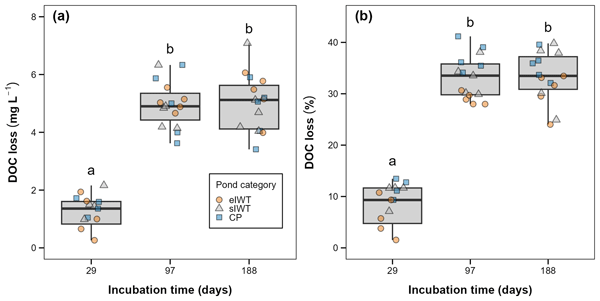
L.250-261. The presentation of DOC loss results (Figure 2) could be clearer, particularly the distinction between differences among pond categories, differences across incubation time, and the nutrient effects (using different colors or shapes in the box plot could help clarify). Are the nutrient-replete samples included in the box plot? Also, why didn’t you include the short-term changes in DOC over 8 days in this box plot? I think either panel A or B would be ok to include in the main text.
RESPONSE: Following these recommendations, we updated Figure 3 (formerly Figure 2) to use distinct colors and shapes for each pond category. Boxplots show only ambient-nutrient samples (one point per pond); nutrient-replete samples are excluded. This is now stated in the figure caption. Incubation times are labeled on the x-axis for clear differentiation. Short-term DOC changes (day 8 to day 29) are not shown in Figure 3 because variability over that interval was minimal; we focused the figure on medium- to long-term trends. Short-term results are provided in Supplement Table S1.
L265. In Figure 1, fluorescence intensity is shown for different components obtained from PARAFAC. Given that DOC concentrations differ among pond categories, it would be helpful to clarify whether differences in Fmax reflect changes in DOM composition or simply differences in overall DOC concentration. Consider presenting the %component to show the relative contributions of components and facilitate the interpretation of compositional differences. The Fmax is of limited use to draw conclusions from since concentration is embedded in the intensity. Since the PARAFAC components are not available to see visually, it is hard to know if two or three of the components are redundant and could be merged into one. Components should always be provided to readers so that they can see their shapes – for example, one can see if they are a single peak or a double peak.
RESPONSE: The spectral characteristics of the components identified by PARAFAC analysis are now provided in the supplement (Figure S1). Following your suggestion, we also present the relative contributions of components in Figure 1 in addition to Fmax.
L.270.Please be consistent in figure names, either figure or fig.
RESPONSE: Figure names are consistent. They are written in full characters in captions and as specified in the guidelines of the journal, the abbreviation "Fig." is used when it appears in running text.
In section 3.3, L278, please state that the results are derived from an exponential model with a residual component. Also, include the justification for choosing this model over others, as noted in the comment above. One strong point of this study is the comparison of model fits. It is useful to give a clear discussion about the advantages or disadvantages of the different models.
RESPONSE: Following one of your recommendations, we previously relocated a paragraph from Section 2.4 to the beginning of Section 3.3. The opening paragraph of Section 3.3 now explicitly states that the results are derived from the exponential model with a residual component (lines 303-305). We believe that discussing the advantages and disadvantages of different model is beyond the scope of our study, as it was not designed for this purpose.
L.285. It would be good to include the statistical results of the linear regression in the SI.
RESPONSE: The statistical results of the linear regressions are now provided in Supplement Table S3.
L.295. Figure 3. Under nutrient-replete conditions, the changes in DOCt/DOC0 appear more variable, particularly among certain eIWT and sIWT ponds. It would be useful to comment on whether these ponds shared any distinctive initial characteristics. Did you statistically check if DOC decomposition varies across pond categories in nutrient addition treatments? This seems to be an important missing analysis.
L.295. Figure 3. Under nutrient-replete conditions, the changes in DOCt/DOC0 appear more variable, particularly among certain eIWT and sIWT ponds. It would be useful to comment on whether these ponds shared any distinctive initial characteristics. Did you statistically check if DOC decomposition varies across pond categories in nutrient addition treatments? This seems to be an important missing analysis.
RESPONSE: This analysis is not missing. In the method section we wrote "In the model, pond category (three levels: eIWT, sIWT or CP) and nutrient addition (two levels: ambient or nutrient-replete) were treated as fixed effects, with pond included as a random effect.". It means that we are testing if DOC decomposition (the k coefficient) is similar among pond categories. In the result we wrote "The interaction between the two factors indicated that the effect of nutrient addition on k depended on pond category (F(2, 181) = 137.1, P = 6.14 × 10⁻²⁴). However, pairwise comparisons did not reveal any differences among group means; the lowest P-value observed was 0.31 for the comparison between unamended eIWT and CP ponds (Figure 4). ".
L.315. Did you consider checking the normalized decay rate over DOC concentration (k/DOC)? This can help eliminate the influence of DOC concentration, as the focus of the study is on evaluating differences in DOM composition.
RESPONSE: The first-order decay coefficient k (in day-1) is independent of DOC concentration in ponds and should not be confused with the DOC decay rate (in e.g., mg C L-1 day-1), which represents an absolute loss rate dependent on the initial DOC concentration. In other words, Equation 3, which is used to estimate k, expresses decay as a fraction of the initial DOC pool.
In Figure 5, please revise the figure caption; the x-axis of the figure 5c needs to be described.
RESPONSE: The caption of the Figure 5 was revised accordingly.
L.309. The discussion refers to water residence time, but it was not directly measured in this study. This connection should therefore be framed more cautiously or supported more explicitly using previous hydrological work at the site.
RESPONSE: Water residence time was not estimated at our study site. This limitation is now acknowledged in the manuscript, where we have provided information on the hydrological connectivity in ponds of the polygonal tundra (Section 4.1, lines 345-349).
L.320. How negligible is this in comparison to this study? Not sure if the dry season could be a good explanation, as drier seasons might increase the WRT and could also reduce terrestrial input. Overall, I think it’s good to discuss more and elaborate further in the discussion.
RESPONSE: In the study by Laurion et al. (2021), DOC loss measured over 12 days was below the 0.5 mg L-1 quantification limit of the TOC analyzer. We observed a DOC loss of 1.0 ± 0.2 mg L-1 over 29 days. These values are comparable and suggest that DOC loss is negligeable when measured during incubations of about month. We have now explicitly noted the DOC loss reported in Laurion et al. (2021) in the revised manuscript.
L.324. Please clarify comparable duration - how many days of incubation?
RESPONSE: Twenty-eight days exactly. This has been clarified in the text (Section 4.1, lines 362-363).
Section 4.1. The authors observed significant differences in DOM composition but similar DOC loss across pond types. It has been discussed that DOC changes over time, and the plateau in DOCt/DOC0 represents the DOM pools, which could be due to the depletion of the labile fraction. Further elaboration on the study results is needed to show that the remaining DOC fraction is mainly from a recalcitrant pool. How do different peaks from fluorescence methods change as the data were collected over different days of incubation?
RESPONSE: Figure S4 illustrates the temporal dynamics of fluorescence intensity for each PARAFAC component during incubation. Only components P1 and P2 show clear changes in intensity. Although it is not possible to definitely assess the nature of the residual DOM solely from our fluorescence data, we did observe an increase in the humification index (HIX; data not presented), consistent with the semi-labile (rather than recalcitrant) nature of the residual DOM pool. We have not revised the manuscript text on this point, however, because as stated in Section 3.3 (lines 305-307), we focused our analysis on k rather than on the residual DOM fraction, and Fig. S4 already provides the requested information on components dynamics.
References
Abbott, B. W., Larouche, J. R., Jones Jr, J. B., Bowden, W. B., & Balser, A. W. (2014). Elevated dissolved organic carbon biodegradability from thawing and collapsing permafrost. Journal of Geophysical Research: Biogeosciences, 119(10), 2049-2063.
Fourrier, P., Dulaquais, G., & Riso, R. (2022). Influence of the conservation mode of seawater for dissolved organic carbon analysis. Marine Environmental Research, 181, 105754.
Kaplan, L. A. (1994). A field and laboratory procedure to collect, process, and preserve fresh‐water samples for dissolved organic carbon analysis. Limnology and Oceanography, 39(6), 1470-1476.
Li, Z., Xu, W., Kang, L., Kuzyakov, Y., Chen, L., He, M., ... & Yang, Y. (2023). Accelerated organic matter decomposition in thermokarst lakes upon carbon and phosphorus inputs. Global Change Biology, 29(22), 6367-6382.
Pacoureau, T., Mazoyer, F., Maranger, R., Rautio, M., and Laurion, I. (2025). Shifts in dissolved organic matter and nutrients in tundra ponds along a gradient of permafrost erosion, Arctic Science, 11, 1-17.
Sinsabaugh, R. L., Hill, B. H., & Follstad Shah, J. J. (2009). Ecoenzymatic stoichiometry of microbial organic nutrient acquisition in soil and sediment. Nature, 462(7274), 795-798.
Vonk, J. E., Tank, S. E., Mann, P. J., Spencer, R. G., Treat, C. C., Striegl, R. G., ... & Wickland, K. P. (2015). Biodegradability of dissolved organic carbon in permafrost soils and aquatic systems: a meta-analysis. Biogeosciences, 12(23), 6915-6930.
Citation: https://doi.org/10.5194/egusphere-2025-5257-AC2
Peer review completion


Interactive discussion
Status: closed
-
RC1: 'Comment on egusphere-2025-5257', Anonymous Referee #1, 11 Feb 2026
Review of the manuscript titled “Bioreactivity of dissolved organic carbon in ponds of the ice-wedge polygonal tundra”, proposed by Thomas Pacoureau, Milla Rautio and Isabelle Laurion.
This study tried to describe processes surrounding the dynamics of the dissolved organic carbon (quantity and quality), specifically for a variety of defrosted Arctic ponds under the short summer season. For this matter, Pacoureau et al. have associated a sampling of environmental reference forcing conditions with a controlled laboratory experiment to reproduce DOC loss over the season under heterotrophic conditions. The experiment is doubled with a nutrient-enriched essay to test the second hypothesis of work on the drivers limiting microbial biomass growth. The dissolved organic carbon is studied under the spectrum of its concentration for the quantitative part and under the spectrum of its optical properties for the qualitative part. Finally, Pacoureau et al. concluded that beyond a homogeneous loss of DOC over ponds and to the end of the season, it is the lability of the DOC that showed correlations with pond-types and the environmental conditions, opening the discussion over global change effects on such ecosystems.
Global critic
Globally, I enjoyed discovering this study, the scientific strategy, its results and the biogeochemical processes finally highlighted. Besides, I found a consistent and well-written text (almost all the time) easy to follow and understand. However, there is for me one structural issue that I will detail below, in addition to minor questions or remarks. To resume the minor remarks, I mainly found terms or phrases vague or ambiguous, needing more precision and justification.
Autotrophic processes and the global carbon cycle
As a scientific strategy, you chose to minimise the autotrophic processes in your experiments, but it must be acknowledged that, finally, the labile OM provided is essential in explaining the DOC loss dynamics. There are structural gaps in its integration of it, from the beginning to the end. As you saw, chlorophyll a levels are quite high, meaning an active local living biomass of phytoplankton, maybe also the mat of cyanobacteria, providing protein-like DOC, and the microbial compartments consumed it preferentially until 90 days (why the plateau?). One parameter, phaeopigments, would have really tested all your grey areas. As a proxy of the decayed photoautotroph cells, it would have better accounted for the cyanobacteria mats (more phaeo than chla since it is not in the water), and quantified the labile POM pool besides the P1-P2 dynamics. Maybe as a hypothesis, all the chla+phaeo have been consumed at D+90 (or is it another nutrient that is limiting? Unfortunately, it's not discussed). Also, there is no discussion about the link between phytoplankton (and microphytobenthos including cyanobacteria) and the bacterial compartment, known to be strongly intricated in quantity and quality (Costas-Selas et al., 2024; Liénart et al., 2020). Finally, I craved for a better discussion integrating the relationships of decreasing decay while a360 increasing, DOC loss and P1 intensity in terms of the global carbon cycle. What do your (great) findings tell us about the carbon qualitative dynamics of the region (4.6 to reshape)? I do not see a clear statement to conclude strongly the discussion, where flux biogeochemists will use your paper(s) to clearly state: What does this new understanding about heterotrophic consumption of DOC tell us about the exchanges between compartments? What is the specific role of such aquatic ecosystems in the global carbon cycle (in view of the current knowledge, Chaplot and Mutema, 2021)? Maybe a conceptual synthesis figure is the only answer to this last point.
Abstract
l.11-12: Maybe the concept of “ice-wedge polygonal tundra” is a little too niche to not be defined even in the abstract. For you to see.
l.18: “in these shallow lentic systems” seems awkward to be recalled here.
l.20: The pond types have to be called at least, and they do not originate from this study, so just call them.
Introduction
l.32-33: Are 5 references really necessary?
l.34: Vegetation has not been introduced yet; it has to be done earlier to understand what primary producers (living or decayed) exist in such a particular ecosystem.
l.47: I suppose you used “watershed” for its American meaning of surface of catchment. I suggest that for all English users, you use a less ambiguous term (catchment, basin, drainage area, etc.).
l.63-64: The description of the three types of ponds is simple and clear, but introduced ambiguously. I don't understand what "representative" means here. You have already established that there are only three types of ponds in these systems, so it seems clearer to me to say "the three types of ponds that can be found in ...".
Material and methods
Study site: I found in Pacoureau et al. 2025 the study site figure I wanted, firstly to understand personally what a polygonal ice-wedge tundra is and what the ponds look like, and secondly to check why there is nothing graphical in this Method. I know that after an analogous paper about the same site, you are tempted to resume the Material and Methods for the next one, but as proof, I was not able to understand this article without seeing the previous one. I would like to see a more detailed description of the study site, something between the actual version and the Pacoureau et al. 2025 one.
MLR: I have some questions about the statistics. Why did you choose to perform only multiple linear regressions, and not general linear models, that would have permitted testing more distributions than the simple Gaussian one, also avoiding the log transformation for scaling? For the multicollinearity, why Spearman and not the Variance Inflation Factor (Borcard et al., 2011)? Why the AIC and not the BIC? You do not mention whether you checked that you retained models only if all the variables were significant. I suggest testing those, or justify why not.
l.83-84: I understand that there is 78 mm of precipitation on average in total over the 3 months. This should be marked more clearly to avoid confusion (with monthly precipitation).
l.106-108: I don’t understand. Smaller than what? I understood above that you used a greater mesh size than usual, to retain more bacteria, but always excluding bacterivores. Either a word is false, or the paragraph should be clearer.
l.112-115: Unless I am mistaken, you are not taking this bias into account in the discussion on the DOC loss.
l.126: naïve question, why a 29-day basis for a month and not 30 or 31?
l.127-128: Please specify the GF75 grade, not to mistake the filter properties with the GF/F one
l.133-135: I suggest displaying the equations as a synthesis, at least for the complex exponential one (which is prominent later).
Results
3.1: Chlorophyll a levels are quite interesting; you should acknowledge them to discuss more about the trophic level later (associated with the nutrient-based part of the discussion). Fmax of microbial-like and protein-like are at the same level, is not it interesting to note it in view of the discussion?
3.2: Good
3.3: Good. I am just wondering if the information carried by the figure 4 is sufficient to be a whole figure, or if it cannot be mixed with fig. 3 or just put as a table.
3.4: As it stands, the figure 6 is badly exploited. I had to go to Pacoureau et al. 2025 to figure out what the EE signature of P1 was, finally to see that the scales are not the same for each pond type. It is not correct. For me, EEMs have a quantitative lecture, so you have to homogenise the scales. Then you will be able to describe it, comparing the ΔRU but also between the ponds.
l.232-233: The form could be better.
Discussion and conclusion
I found the discussion pleasant, well-structured and written, outside of the global criticism.
L389-390: You should check your writing around the nutrient mentions (here the C:N and C:P ratios), where you forget to mention “dissolved”, I know that it seems obvious for you, but not for those who juggle between dissolved and particulate.
4.5: I find this part of the discussion a bit too advanced (l.410-411), as you voluntarily focused your experiments on the heterotrophic processes; even if you have found a great residual DOC pool, you don’t know the amplitude of action of photodegradation and primary production, for example. Independently, some insights about what forcings can be responsible for resuspension (l.414-415) will deepen this paragraph.
l.426-427: the reverse is also true from POM to DOM (Hu et al., 2022).
l.439: The first sentence of the conclusion is decisive, and it should be more precise. I suggest either adding a bio-essay (or experiment) around or replacing “estimation”, and/or adding heterotrophic or microbial to “DOM decomposition”.
l.420: As for the abstract, I do not understand your use of “morphological” and “limnological”, terms that are vague to me. I found in your article a comparison of pond types, led by their hydro(geo)morphology, and a comparison of nutrient levels, so biogeochemistry.
Suggestion to the editor
As a synthesis, I found that the science carried by this manuscript, after intermediary corrections, will be a matter of interest and advances and should be disseminated to the scientific community in this journal.
References
Borcard, D., Legendre, P., and Gillet, F.: Numerical Ecology with R, Springer, 315 pp., 2011.
Chaplot, V. and Mutema, M.: Sources and main controls of dissolved organic and inorganic carbon in river basins: A worldwide meta-analysis, Journal of Hydrology, 603, 126941, https://doi.org/10.1016/j.jhydrol.2021.126941, 2021.
Costas-Selas, C., Martínez-García, S., Delgadillo-Nuño, E., Justel-Díez, M., Fuentes-Lema, A., Fernández, E., and Teira, E.: Linking the impact of bacteria on phytoplankton growth with microbial community composition and co-occurrence patterns, Marine Environmental Research, 193, 106262, https://doi.org/10.1016/j.marenvres.2023.106262, 2024.
Hu, B., Wang, P., Wang, C., and Bao, T.: Photogeochemistry of particulate organic matter in aquatic systems: A review, Science of The Total Environment, 806, 150467, https://doi.org/10.1016/j.scitotenv.2021.150467, 2022.
Liénart, C., Savoye, N., Conan, P., David, V., Barbier, P., Bichon, S., Charlier, K., Costes, L., Derriennic, H., Ferreira, S., Gueux, A., Hubas, C., Maria, E., and Meziane, T.: Relationship between bacterial compartment and particulate organic matter (POM) in coastal systems: An assessment using fatty acids and stable isotopes, Estuarine, Coastal and Shelf Science, 239, 106720, https://doi.org/10.1016/j.ecss.2020.106720, 2020.
Citation: https://doi.org/10.5194/egusphere-2025-5257-RC1 -
AC1: 'Reply on RC1', Thomas Pacoureau, 15 May 2026
We sincerely appreciate the time and effort you have dedicated to reviewing our manuscript. Your comments and suggestions have been invaluable in improving the clarity and robustness of our study. We have carefully addressed each point and incorporated the necessary revisions accordingly. Below, we provide a detailed response to all comments.
1. Global critic: autotrophic processes and the global carbon cycle
COMMENT: As a scientific strategy, you chose to minimise the autotrophic processes in your experiments, but it must be acknowledged that, finally, the labile OM provided is essential in explaining the DOC loss dynamics. There are structural gaps in its integration of it, from the beginning to the end. As you saw, chlorophyll-a levels are quite high, meaning an active local living biomass of phytoplankton, maybe also the mat of cyanobacteria, providing protein-like DOC, and the microbial compartments consumed it preferentially until 90 days (why the plateau?). One parameter, phaeopigments, would have really tested all your grey areas. As a proxy of the decayed photoautotroph cells, it would have better accounted for the cyanobacteria mats (more phaeo than chla since it is not in the water), and quantified the labile POM pool besides the P1-P2 dynamics. Maybe as a hypothesis, all the chla+phaeo have been consumed at D+90 (or is it another nutrient that is limiting? Unfortunately, it's not discussed). Also, there is no discussion about the link between phytoplankton (and microphytobenthos including cyanobacteria) and the bacterial compartment, known to be strongly intricated in quantity and quality (Costas-Selas et al., 2024; Liénart et al., 2020).
RESPONSE: The reviewer raised a concern regarding the lack of integration of autotrophic processes in our experiment. Dark bottle incubations (isolated from benthic processes) are specifically intended to suppress DOC production via photosynthesis. Although this approach has limitations, this step is essential for isolating and quantifying DOC consumption by planktonic heterotrophic activity, and it is a well-established method for assessing the lability or decay of DOM present in the environment at a specific time. We are therefore uncertain that we fully understand how integrating autotrophic processes would benefit our primary objectives: to compare estimates of DOM bioavailability across pond types, and to explore their relationship with specific DOM components.
To consider the effect of autotrophic processes on DOM decomposition dynamics along a dark incubation, shorter incubation times (e.g., a few hours or a day) would be needed to reflect the decomposition rates of labile DOM by bacteria, provided that DOC decline can be quantified, though measurements for this approach are not sensitive enough. Alternatively, a light-exposed continuous bioreactor with repeated sampling to measure DOM loss/decay in dark bottle incubations at several time points could be considered. However, such an experiment presents conceptual challenges in capturing the influence of benthic primary producers, which appear to be the dominant source of autotrophic DOM in tundra ponds. Additionally, replicating in situ light conditions in these incubations would be technically difficult due to the strong variability in light exposure within and across ponds. Although interactions between bacteria and phytoplankton influence bacterial activity (e.g., predation by mixotrophic algae, competition for nutrients, production of metabolites), we consider that discussing the link between phytoplankton/microphytobenthos and the bacterial compartment is beyond the scope of our experiment.
We did not monitor algal biomass, nor pigment decay as pheophytin-a, during incubations. We did however obtain indirect estimates of photoautotrophic decay at t0 of the incubation through measurements of phaeophytin-a (the most abundant phaeopigment): our analytical method corrects chlorophyll-a (Chla) concentrations for the presence of pheophytin-a (Pheo), providing insights into the degradation status of algal cells. While Chla ranged from 0.3 to 12.6 µg L-1 (avg = 2.95 µg L-1; median=1.9 µg L-1; range without the max value 0.3–6.7 µg L-1) and Pheo from 0.3 to 1.6 µg L-1, the Pheo:Chla ratio in our samples ranged from 0.3 to 1.2 (mean = 0.6). Notably, the lowest ratios (i.e., less degraded communities) were observed in samples where Chla exceeded 1.5 µg L⁻¹, likely reflecting more active or recently produced algal biomass. These values suggest that the proportion of decayed photoautotrophic cells relative to total algal biomass was fairly high at sampling. It should be noted that at these low biomass ranges, errors can be large for this ratio. In conclusion, we are not convinced that Pheo has the potential to address all the concerns mentioned by the reviewer.
In the revised manuscript, we now highlight the presence of Chla as a predictor in the second-best models for DOC loss (Section 3.4, lines 319-321), and discuss the potential enhancement of DOC decay driven by labile DOM produced by living and senescent phytoplanktonic and benthic cells at the onset of incubations (Section 4.4, lines 466-476).
COMMENT: Finally, I craved for a better discussion integrating the relationships of decreasing decay while a360 increasing, DOC loss and P1 intensity in terms of the global carbon cycle. What do your (great) findings tell us about the carbon qualitative dynamics of the region (4.6 to reshape)? I do not see a clear statement to conclude strongly the discussion, where flux biogeochemists will use your paper(s) to clearly state: What does this new understanding about heterotrophic consumption of DOC tell us about the exchanges between compartments? What is the specific role of such aquatic ecosystems in the global carbon cycle (in view of the current knowledge, Chaplot and Mutema, 2021)? Maybe a conceptual synthesis figure is the only answer to this last point.
RESPONSE: To address this comment, we expanded the discussion (Section 4.6, lines 511-513) and the conclusion (Section 5, lines 534-536). We respectfully disagree that a conceptual synthesis figure is necessary for this manuscript.
Regarding the reviewer's request to situate our findings within the global carbon cycle: While we appreciate the suggestion to contextualize our results in terms of global carbon dynamics, we believe such extrapolation would be premature and potentially misleading given the scope and design of our study. Chaplot and Mutema (2021) conduct a global-scale meta-analysis of riverine inorganic and organic carbon fluxes, a fundamentally different system and spatial scale than our study of small polygonal tundra ponds. Direct comparison or integration with such global flux assessments is not straightforward. Specifically, several methodological and conceptual challenges prevent robust upscaling of our findings:
(1) Our bioassays quantified DOC consumption by heterotrophic bacteria but did not directly measure CO₂ mineralization. Converting observed decay coefficients to areal or volumetric carbon fluxes (e.g., g C m⁻² d⁻¹) would require assumptions about respiratory quotients, mineralization efficiency, and in situ bacterial production rates, none of which were measured in this study.
(2) Spatial extrapolation is constrained by the lack of comprehensive geospatial data on the areal extent of ice-wedge tundra ponds across the Arctic. Even within well-studied regions, classification and mapping of eIWT, sIWT, and CP pond types remain incomplete, making landscape-scale or regional carbon budget estimates highly uncertain.
Our primary objective was to compare DOM bioreactivity across geomorphologically distinct pond types and identify the compositional drivers of decomposition, not to provide global carbon cycle estimates. We believe our findings contribute valuable mechanistic insights that can inform future synthesis efforts as spatial data and process-based models improve. We have clarified this scope in the revised discussion.
2. Abstract
l.11-12: Maybe the concept of “ice-wedge polygonal tundra” is a little too niche to not be defined even in the abstract. For you to see.
RESPONSE: Following the recommendation, we adjusted the abstract to clarify (Abstract, lines 12-13).
l.18: “in these shallow lentic systems” seems awkward to be recalled here.
RESPONSE: We addressed this by rephrasing the passage for clarity (Abstract, lines 14-18).
l.20: The pond types have to be called at least, and they do not originate from this study, so just call them. RESPONSE: We added the names of the ponds in parentheses (Abstract, lines 20-21).
3. Introduction
l.32-33: Are 5 references really necessary?
RESPONSE: We limited the references to the three most recent ones to support our argument (Section 1, lines 31-32).
l.34: Vegetation has not been introduced yet; it has to be done earlier to understand what primary producers (living or decayed) exist in such a particular ecosystem.
RESPONSE: We now include such a description, and extended our presentation of primary producers to phytoplankton and benthic cyanobacterial mats (Section 1, lines 35-38). We also added a short description of the vegetation at the study site in the method section (Section 2.1, lines 93-99).
l.47: I suppose you used “watershed” for its American meaning of surface of catchment. I suggest that for all English users, you use a less ambiguous term (catchment, basin, drainage area, etc.).
RESPONSE: We replaced "watershed" by "catchment" as suggested (Section 1, line 55).
l.63-64: The description of the three types of ponds is simple and clear, but introduced ambiguously. I don't understand what "representative" means here. You have already established that there are only three types of ponds in these systems, so it seems clearer to me to say "the three types of ponds that can be found in ...".
RESPONSE: We and rephrased the sentence accordingly (Section 1, lines 74-76).
4. Material and methods
COMMENT: Study site: I found in Pacoureau et al. 2025 the study site figure I wanted, firstly to understand personally what a polygonal ice-wedge tundra is and what the ponds look like, and secondly to check why there is nothing graphical in this Method. I know that after an analogous paper about the same site, you are tempted to resume the Material and Methods for the next one, but as proof, I was not able to understand this article without seeing the previous one. I would like to see a more detailed description of the study site, something between the actual version and the Pacoureau et al. 2025 one.
RESPONSE: To assist readers unfamiliar with this type of landscape, we deemed it useful to include photographs of the study site and ponds representative of the categories discussed in the article (new Figure 1). The description of the ponds has also been expanded in the text (Section 2.1, lines 106-116).
COMMENT: MLR: I have some questions about the statistics. Why did you choose to perform only multiple linear regressions, and not general linear models, that would have permitted testing more distributions than the simple Gaussian one, also avoiding the log transformation for scaling? For the multicollinearity, why Spearman and not the Variance Inflation Factor (Borcard et al., 2011)? Why the AIC and not the BIC? You do not mention whether you checked that you retained models only if all the variables were significant. I suggest testing those, or justify why not.
RESPONSE: We address each of these questions separately below.
1/ Why did you choose to perform only multiple linear regressions, and not general linear models, that would have permitted testing more distributions than the simple Gaussian one, also avoiding the log transformation for scaling?
RESPONSE: We think that the reviewer wanted to write "generalized linear models" instead of "general linear models". As specified in the third paragraph of the Section Statistical analysis, we log-transformed some of the explanatory variables (S285, Chla, and P2). The response variables however, either DOC loss at day 97 or 188 or decay coefficient, were not transformed. We acknowledge that no transformation was necessary for the explanatory variables to use linear regression in the first place. We now use untransformed variables.
The question regarding the choice of linear models over generalized linear models remains valid. Upon examining the residual patterns from the linear models, we observed no clear violations of normality or heteroscedasticity. Consequently, we were not inclined to refit our data using GLMs.
When we reanalyzed the data using GLMs with two link functions from the Gamma family, the log-normal and Gamma distributions (potentially well-suited for DOC decomposition in batch experiments, given their continuous, non-zero, and right-skewed nature), we found not improvement in diagnostic plots or residual heteroscedasticity. The best GLM-selected models for explaining DOC loss at days 97 and 188 still included only the initial (t₀) fluorescence intensity of the PARAFAC component P1. These findings further support that our linear regression approach is well-suited to this dataset.
2/ For the multicollinearity, why Spearman and not the Variance Inflation Factor (Borcard et al., 2011)?
RESPONSE: The final sets of explanatory variables are consistent between the two methods (Spearman and VIF with a cutoff of 10), with one exception: in the VIF-based selection, a320 is replaced by HT4. Given that a320 serves as a strong proxy for the fluorescence intensity of all PARAFAC components (Spearman’s ρ > 0.9) and that the VIF values for all variables retained via the Spearman-based approach are ≤ 10, we opt to retain the original selection method.
3/ Why the AIC and not the BIC?
RESPONSE: While both AICc and BIC have advantages and limitations in this context, we selected AICc because BIC’s assumption (that the true model is included in the candidate set) is unlikely to hold here. Additionally, BIC’s stronger penalty for complexity increases the risk of underfitting. Nevertheless, both criteria ultimately converged on the same optimal model.
4/ You do not mention whether you checked that you retained models only if all the variables were significant.
RESPONSE: The only variable consistently significant (P < 0.05) across all AICc-selected models was P1. This supports the choice for the model we present (a linear regression of initial P1 intensity against DOC loss). We have incorporated this clarification into the manuscript (Section 2.8, lines 250-252 and Section 3.4, lines 321-322).
l.83-84: I understand that there is 78 mm of precipitation on average in total over the 3 months. This should be marked more clearly to avoid confusion (with monthly precipitation).
RESPONSE: We addressed this by rephrasing the passage for clarity (Section 2.1, lines 91-93).
l.106-108: I don’t understand. Smaller than what? I understood above that you used a greater mesh size than usual, to retain more bacteria, but always excluding bacterivores. Either a word is false, or the paragraph should be clearer.
RESPONSE: We addressed this by rephrasing the passage for clarity (Section 2.3, lines 127-128).
l.112-115: Unless I am mistaken, you are not taking this bias into account in the discussion on the DOC loss.
RESPONSE: We now examine the potential effects of temperature differences between incubation and in situ conditions (Section 4.1, lines 390-395). For this analysis, we assumed a Q10 value of 2. We also adjusted the text to account for natural thermal fluctuations in this type of system (Section 4.1, lines 395-398).
l.126: naïve question, why a 29-day basis for a month and not 30 or 31?
RESPONSE: A standard basis for the duration of bioassays is 28 days. Sampling on the 28th day would have been ideal for comparison of our results with other studies. Unfortunately, this was not feasible due to logistical constraints.
l.127-128: Please specify the GF75 grade, not to mistake the filter properties with the GF/F one.
RESPONSE: We replaced "grade F" by "GF75" as suggested (Section 2.4, lines 150-151).
l.133-135: I suggest displaying the equations as a synthesis, at least for the complex exponential one (which is prominent later).
RESPONSE: Equations have been added as suggested in the Section 2.4 (lines 159-167).
5. Results
COMMENT: 3.1: Chlorophyll a levels are quite interesting; you should acknowledge them to discuss more about the trophic level later (associated with the nutrient-based part of the discussion). Fmax of microbial-like and protein-like are at the same level, is not it interesting to note it in view of the discussion?
RESPONSE: We agree that chlorophyll concentrations are an important indicator of trophic conditions. However, we caution that assessing the trophic status of the ponds based on single-point sampling provides limited insight for a robust discussion. While Table 1 reports a chlorophyll a (Chla) concentration range of 0.3–12.6 µg L⁻¹, excluding the maximum value reduces the range to 0.3–6.7 µg L⁻¹, suggesting that most observations fall within the lower end of the reported spectrum. That said, we acknowledge that these values remain consistent with productive systems. Primary production by both macrophytes and phytoplankton in these warm, shallow, and nutrient-rich water bodies (Table 1) is therefore likely to influence carbon cycling, notably by enhancing atmospheric CO₂ uptake and contributing inputs of recently fixed carbon. We have added a sentence to clarify this point in the discussion (Section 4.4, lines 468-471).
With respect to the roughly equivalent fluorescence levels between microbial-like and protein-like components: one possible hypothesis is that microbial production of FDOM is associated with protein-like FDOM levels in these ponds. However, we currently lack sufficient evidence to explore this relationship further in the discussion. All FDOM components could be considered “microbial” from a certain perspective (from bacteria, archaea, fungi, and protozoans), making these names used in the literature potentially misleading.
COMMENT: 3.3: Good. I am just wondering if the information carried by the figure 4 is sufficient to be a whole figure, or if it cannot be mixed with fig. 3 or just put as a table.
RESPONSE: Thank you for the suggestion. The two figures were combined into a single one (new Figure 4).
COMMENT: 3.4: As it stands, the figure 6 is badly exploited. I had to go to Pacoureau et al. 2025 to figure out what the EE signature of P1 was, finally to see that the scales are not the same for each pond type. It is not correct. For me, EEMs have a quantitative lecture, so you have to homogenise the scales. Then you will be able to describe it, comparing the ΔRU but also between the ponds.
RESPONSE: We acknowledge that EEMs provide a quantitative information. For the right panel of Figure 6 showing ΔRU, we have standardized the color scales to facilitate comparison of fluorescence changes across the three ponds (note that these represent individual examples per category rather that mean decreases). However, for the left panel, we retained the original scales to effectively illustrate differences between t0 and t188. Homogenizing these scales would obscure important variations in fluorescence intensity among ponds due to their substantial baseline differences. To enhance interpretation of figure 6, we added the P1 peak excitation-emission maxima. The signature of P1 is now visible on figure S1 in the supplement along with the spectral characteristics of the other PARAFAC components.
l.232-233: The form could be better.
RESPONSE: We addressed this by rephrasing the passage for clarity (Section 3.1, lines 260-262).
6. Discussion and conclusion
L389-390: You should check your writing around the nutrient mentions (here the C:N and C:P ratios), where you forget to mention “dissolved”, I know that it seems obvious for you, but not for those who juggle between dissolved and particulate.
RESPONSE: The ratios in question are actually DOC:TN and DOC:TP, which we have now denoted as such in the text (Section 4.3, line 436 and lines 446-448) and the new Table 1 to address this comment. The validity of using such ratios is supported by data in Pacoureau et al. (2025): 93% of TN occurs in the form of NH4+, and although orthophosphates comprise only 30% of TP, phosphorus is rapidly cycled in the studied ponds, making TP a reasonable proxy for bioavailable P.
COMMENT: 4.5: I find this part of the discussion a bit too advanced (l.410-411), as you voluntarily focused your experiments on the heterotrophic processes; even if you have found a great residual DOC pool, you don’t know the amplitude of action of photodegradation and primary production, for example. Independently, some insights about what forcings can be responsible for resuspension (l.414-415) will deepen this paragraph.
RESPONSE: We have now mentioned photomineralization in the paragraph as a process that may act on the residual pool observed in our dark incubations, and adjusted the text to clarify that resuspension would occur during mixing periods for such stagnant waterbodies (Section 4.5, lines 483-484). We believe this discussion is useful and not overly extensive (11 lines), and addresses an important question: the fate of the DOC pool not consumed after 100 days.
l.426-427: the reverse is also true from POM to DOM (Hu et al., 2022).
RESPONSE: Our intention was to present factors responsible for the removal of DOM. We rephrased for better clarity (Section 4.6, lines 493-494).
l.439: The first sentence of the conclusion is decisive, and it should be more precise. I suggest either adding a bio-essay (or experiment) around or replacing “estimation”, and/or adding heterotrophic or microbial to “DOM decomposition”.
RESPONSE: We addressed this by rephrasing the passage for clarity (Section 5, lines 519-520).
l.420: As for the abstract, I do not understand your use of “morphological” and “limnological”, terms that are vague to me. I found in your article a comparison of pond types, led by their hydro(geo)morphology, and a comparison of nutrient levels, so biogeochemistry.
RESPONSE: The abstract has been corrected to state that hydro-morphological processes are responsible for the diversity of ponds (Abstract, lines 12-14). We also replaced the term "limnological" lines 86 and 420 by "biogeochemical", which seems better suited (Section 2.1, lines 105-106 and Section 4.6, lines 490-491).
Citation: https://doi.org/10.5194/egusphere-2025-5257-AC1
-
AC1: 'Reply on RC1', Thomas Pacoureau, 15 May 2026
-
RC2: 'Comment on egusphere-2025-5257', Anonymous Referee #2, 17 Mar 2026
Manuscript review:
Bioreactivity of dissolved organic carbon in ponds of the ice-wedge polygonal tundra
General description:
This manuscript investigates the bioreactivity of dissolved organic carbon (DOC) in ponds located within ice-wedge polygonal tundra landscapes on Bylot Island (Canadian Arctic). The authors conducted an 188-day dark incubation experiment using water from 15 ponds representing three geomorphological pond types (eroding ice-wedge troughs, stabilized ice-wedge troughs, and coalescent polygon ponds). Dissolved organic matter (DOM) composition was characterized using absorbance and fluorescence spectroscopy. The components from a PARAFAC analysis in a previous study were used here, identifying eight fluorescent components. DOC degradation dynamics were evaluated using several decay models, including linear, exponential, exponential with residual pool, and gamma reactivity continuum models. The results show that approximately one third of DOC was degraded within 97 days, but no significant differences in DOC loss were observed among pond categories despite differences in DOM optical properties. Nutrient addition did not significantly enhance DOC degradation, and regression analyses suggest that tryptophan-like fluorescence is associated with higher DOC loss.
Overall, the study addresses an important topic in Arctic carbon cycling, particularly the role of thaw ponds in processing permafrost-derived organic matter. The long incubation period is a notable strength, as we expect a warmer climate with lower precipitation and with longer water residence time. The study is generally well explained, and most sections are clear; however, there are a few instances where further explanation is necessary. It would be good to include estimates of short-term (8-day) decay rates, as they provide valuable input for examining the fast pool of DOM. The discussion would benefit from elaborating upon long-term versus short-term degradation rates (Check the paper by Francois Guillemette et al. 2011) and how different model fittings/comparisons between them help interpret observed trends.
There are some aspects of the experimental design and interpretation of the results that would benefit from clarification or additional discussion. I found the methods section harder to follow, especially regarding the replicates, nutrient-addition treatments, and sample size. Please be clear in figure captions to mention how many samples are included in each grouping. In the discussion, the interpretation of the results could be further developed, rather than primarily restating the findings, and some parts of the reasoning need to be improved.
One important component of the study is the characterization of DOM composition using PARAFAC analysis. It was not entirely clear at first that the PARAFAC model was developed with a larger sample size. The sample size of this dataset is small, but it would be helpful to clarify how many samples from the present study were included in the larger PARAFAC model and how many samples in total were included in the PARAFAC modelling. It would be helpful to see the components in the supplementary information. The current analysis of components based on the maximum fluorescence intensity is limited since fluorescence intensity is highly correlated to DOC concentration. Using the %components would be more suitable for assessing the influence of DOM composition and would exclude the effect of DOC concentration.
Finally, it would be valuable to check the nutrient stoichiometry (C:N and C:P) ratio and its potential impact on the degradation rate of DOC. The study finds that nutrient addition did not increase degradation rates. It could help elevate the discussion by explaining how nutrient stoichiometry in these Arctic systems relates to bacterial stoichiometry and by discussing which nutrients might have been more limiting. For example, see Goodwin et al., 2017 – Ecology 98(3):820-829. doi: 10.1002/ecy.1705.
More detailed comments:
L31. Please specify which Arctic regions or landscape types are being referenced here, as DOM sources and processing pathways can vary substantially among Arctic environments.
L40. Please ensure consistent terminology for the optical techniques. Consider using absorbance instead of absorption.
L40. Absorbance and fluorescence spectroscopy are useful tools for characterizing DOM from different sources, including terrestrial and microbially derived DOM (McKnight et al, 2001; Jaffe, 2008). What do you mean by functional properties? Optical characteristics should not be interpreted beyond their original intention. The PARAFAC components can be related to functional characteristics measured across an experimental gradient, but the components themselves are statistical products of a dataset and identify regions of the EMM that covary within a particular dataset. Is the focus of this study explicitly emphasized in the relationship between different DOM fractions and their bioreactivity?
L42. Since the manuscript later relates protein-like fluorescence to DOC bioreactivity, it would be useful to reference previous studies linking tryptophan-like or tyrosine-like fluorescence components to bioavailable DOM.
L.42. What do you mean by synergetic permafrost deposits? It would be helpful to add one sentence for non-specialists to explain this terminology.
L49. Please check spacing
L67. Please clarify how hydrological connectivity was assessed or inferred for the different pond categories, particularly for coalescent polygon ponds.
L70. I am not sure how the first hypothesis was formulated. Could you provide references here? Thawing the surrounding soil releases DOM from soil pores that were previously trapped there, and this may increase the DOM with a terrestrial signature. So, it is expected that the increase of this fraction reduces the bioreactivity.
L116. The description of the bioassay design does not clearly specify the number of incubation units and the replication structure. In particular, it is unclear how many replicate bottles were incubated per sample, how many were nutrient-amended versus unamended, and whether nutrient additions were applied in parallel to control incubations for each sample. The term “replicate incubation units” is introduced without prior definition. Please clarify the number of replicates per treatment and provide a concise summary of the experimental design (e.g., n per treatment, ± nutrient additions). It should be clear to the reader how many samples were included in each analysis and is included in each figure.
L.118. Please explain here the rationale for the selected concentrations of the nutrient additions.
L.120. Is there a reason that 188 days was chosen as the final incubation time? As it is longer than one growing season.
L.129. Were the samples acidified for storage, and if so, how long were the samples stored before analysis? Or alternatively, was the measurement done right after adding the acid? Was any flocculation observed in the samples due to changes in pH, and how long were the samples kept before DOC analysis? A pH of 2 is very low, and some fraction of the DOM is likely to become insoluble if there is a long delay between adding acid and the measurement. Please clarify this section of text.
L145. In the reactivity continuum model, υ describes the shape of a continuous reactivity distribution and the relative contribution of slower-reacting compounds, not a direct measure of abundance or fraction in DOC pools. Clarification or more cautious wording would be appropriate.
L148-154. The last paragraph in section 2.4 is more about results than the method section. It can be moved to section 3.3.
L155. Please state the sample storage duration prior to DOM optical analyses.
L.170. I understand that PARAFAC analysis was done in a previous study (Pacoureau et al 2025), but the explanation could be clearer (e.g., sample size of the larger dataset and a description of the larger dataset). How was the existing parafac model done? Please provide the PARAFAC components in the supplementary information. This section could be explained more clearly since the dataset in this study is small relative to the number of derived components.
L.195-199. The multiple linear regression analyses based on pooled data from 15 ponds and all-subsets model selection are potentially sensitive to overfitting and multicollinearity. As there is strong covariance among DOM optical and chemical predictors, a multivariate approach such as partial least squares regression (PLSR), with appropriate cross-validation, may provide a more robust alternative for relating initial DOM properties to DOC loss metrics.
L.200. I wonder if a mixed-effect model would be more appropriate than two-way mixed measures ANOVA, as there is a repeated measure structure? Please explain the motivation for the decision.
L.226. Consider altering the title. The current title does not clearly reflect questions related to nutrient additions, pond types and DOM composition.
L.245. Could you also include pH, C:N, and C:P ratios in Table 1? It would be useful to examine the stoichiometry and compare with other studies in the discussion. Particularly in reference to the discussion about why nutrient additions did not influence bioreactivity.
L.240. In general, the DOM composition is not statistically different in SIWT and CP for all components except HT2. It is interesting that microbial humic-like is higher in eIWT with a higher tryptophan peak in P1. And in general, the mean of the protein-like component is not different among them. This could be explained more in the discussion. Can it be due to more DOM degradation in eIWT ponds? It could help refine the interpretation of DOM sources and processing.
L.250-261. The presentation of DOC loss results (Figure 2) could be clearer, particularly the distinction between differences among pond categories, differences across incubation time, and the nutrient effects (using different colors or shapes in the box plot could help clarify). Are the nutrient-replete samples included in the box plot? Also, why didn’t you include the short-term changes in DOC over 8 days in this box plot? I think either panel A or B would be ok to include in the main text.
L265. In Figure 1, fluorescence intensity is shown for different components obtained from PARAFAC. Given that DOC concentrations differ among pond categories, it would be helpful to clarify whether differences in Fmax reflect changes in DOM composition or simply differences in overall DOC concentration. Consider presenting the %component to show the relative contributions of components and facilitate the interpretation of compositional differences. The Fmax is of limited use to draw conclusions from since concentration is embedded in the intensity. Since the PARAFAC components are not available to see visually, it is hard to know if two or three of the components are redundant and could be merged into one. Components should always be provided to readers so that they can see their shapes – for example, one can see if they are a single peak or a double peak.
L.270.Please be consistent in figure names, either figure or fig
In section 3.3, L278, please state that the results are derived from an exponential model with a residual component. Also, include the justification for choosing this model over others, as noted in the comment above. One strong point of this study is the comparison of model fits. It is useful to give a clear discussion about the advantages or disadvantages of the different models.
L.285. It would be good to include the statistical results of the linear regression in the SI
L.295. Figure 3. Under nutrient-replete conditions, the changes in DOCt/DOC0 appear more variable, particularly among certain eIWT and sIWT ponds. It would be useful to comment on whether these ponds shared any distinctive initial characteristics. Did you statistically check if DOC decomposition varies across pond categories in nutrient addition treatments? This seems to be an important missing analysis.
L.295. Figure 3. Please display the observed DOCt/DOC0 data points together with the fitted decay curves. Currently, the reader only sees the fitted curve. Without the data points, it’s hard to visualize how well the model fits the experimental data.
L.315. Did you consider checking the normalized decay rate over DOC concentration (k/DOC)? This can help eliminate the influence of DOC concentration, as the focus of the study is on evaluating differences in DOM composition.
In Figure 5, please revise the figure caption; the x-axis of the figure 5c needs to be described
L.309. The discussion refers to water residence time, but it was not directly measured in this study. This connection should therefore be framed more cautiously or supported more explicitly using previous hydrological work at the site.
L.320. How negligible is this in comparison to this study? Not sure if the dry season could be a good explanation, as drier seasons might increase the WRT and could also reduce terrestrial input. Overall, I think it’s good to discuss more and elaborate further in the discussion.
L.324. Please clarify comparable duration - how many days of incubation?
Section 4.1. The authors observed significant differences in DOM composition but similar DOC loss across pond types. It has been discussed that DOC changes over time, and the plateau in DOCt/DOC0 represents the DOM pools, which could be due to the depletion of the labile fraction. Further elaboration on the study results is needed to show that the remaining DOC fraction is mainly from a recalcitrant pool. How do different peaks from fluorescence methods change as the data were collected over different days of incubation?
References:
Guillemette, F., & del Giorgio, P. A. (2011). Reconstructing the various facets of dissolved organic carbon bioavailability in freshwater ecosystems. Limnology and Oceanography, 56(2), 734-748.
McKnight, D. M., Boyer, E. W., Westerhoff, P. K., Doran, P. T., Kulbe, T., & Andersen,
- T. (2001). Spectrofluorometric characterization of dissolved organic matter for indication of precursor organic material and aromaticity. Limnology and Oceanography, 46(1), 38-48.
Jaffé, R., McKnight, D., Maie, N., Cory, R., McDowell, W. H., & Campbell, J. L. (2008). Spatial and temporal variations in DOM composition in ecosystems: The importance of long-term monitoring of optical properties. Journal of Geophysical Research: Biogeosciences, 113(G4), 4032.
Goodwin et al., 2017 Growth rate and resource imbalance interactively control biomass stoichiometry and elemental quotas of aquatic bacteria Ecology 98(3):820-829. doi: 10.1002/ecy.1705.
Citation: https://doi.org/10.5194/egusphere-2025-5257-RC2 -
AC2: 'Reply on RC2', Thomas Pacoureau, 15 May 2026
We are truly grateful for the time and thoughtful consideration you’ve given to our manuscript. Your feedback has greatly strengthened our work, and we have carefully revised the paper in response to your comments. Our replies to each of your suggestions are included below.
COMMENT: There are some aspects of the experimental design and interpretation of the results that would benefit from clarification or additional discussion. I found the methods section harder to follow, especially regarding the replicates, nutrient-addition treatments, and sample size. Please be clear in figure captions to mention how many samples are included in each grouping. In the discussion, the interpretation of the results could be further developed, rather than primarily restating the findings, and some parts of the reasoning need to be improved.
RESPONSE: In response to the global critic, we carefully revised the method section and figure captions to provide a clear picture of the number of samples used during the bioassay. Changes can be seen notably at line 124 and lines 137-138 (Section 2.1) and caption of Figure 3.
COMMENT: One important component of the study is the characterization of DOM composition using PARAFAC analysis. It was not entirely clear at first that the PARAFAC model was developed with a larger sample size. The sample size of this dataset is small, but it would be helpful to clarify how many samples from the present study were included in the larger PARAFAC model and how many samples in total were included in the PARAFAC modelling. It would be helpful to see the components in the supplementary information. The current analysis of components based on the maximum fluorescence intensity is limited since fluorescence intensity is highly correlated to DOC concentration. Using the %components would be more suitable for assessing the influence of DOM composition and would exclude the effect of DOC concentration.
RESPONSE: We brought precision on the dataset used for the development of the PARAFAC model, including the number of samples from this study (Section 2.5, l. 193-196).
COMMENT: Finally, it would be valuable to check the nutrient stoichiometry (C:N and C:P) ratio and its potential impact on the degradation rate of DOC. The study finds that nutrient addition did not increase degradation rates. It could help elevate the discussion by explaining how nutrient stoichiometry in these Arctic systems relates to bacterial stoichiometry and by discussing which nutrients might have been more limiting. For example, see Goodwin et al., 2017.
RESPONSE: Molar C:N and C:P ratios are now presented in Table 1. They are similar to the ratios found in a previous study of the same ponds (Pacoureau et al., 2025). We believe that assessing nutrient limitation in such C-rich systems would require dedicated experiments such as nutrient-enrichment bioassays with factorial N and P additions (e.g., as in Li et al., 2023), or measurement of extracellular enzyme activities coupled with bacterial production assays (e.g., as in Sinsabaugh et al., 2009). The reference provided by the reviewer presents stoichiometric ratios for microbial biomass of 70:13:1 and 73:14:1 (C:N:P). These ratios correspond to two strains under optimal growth conditions, but the authors do not provide sufficient details on how they were estimated. In our view, comparing bacterial stoichiometry from such an experimental study with what we observed in the ponds is not straightforward, and the resulting discussion would be overly speculative.
L31. Please specify which Arctic regions or landscape types are being referenced here, as DOM sources and processing pathways can vary substantially among Arctic environments.
RESPONSE: We specified the Arctic regions under study in the cited reference (Section 1, lines 32-33).
L40. Please ensure consistent terminology for the optical techniques. Consider using absorbance instead of absorption.
RESPONSE: We reviewed the terminology used throughout the text. The terms "absorption spectroscopy" and "absorption coefficient" (e.g., a320) are valid. The absorption coefficient (lowercase a) is derived from absorbance (capital A), which is measured using a spectrophotometer.
L40. Absorbance and fluorescence spectroscopy are useful tools for characterizing DOM from different sources, including terrestrial and microbially derived DOM (McKnight et al, 2001; Jafe, 2008). What do you mean by functional properties? Optical characteristics should not be interpreted beyond their original intention. The PARAFAC components can be related to functional characteristics measured across an experimental gradient, but the components themselves are statistical products of a dataset and identify regions of the EMM that covary within a particular dataset. Is the focus of this study explicitly emphasized in the relationship between different DOM fractions and their bioreactivity?
RESPONSE: We used the term "functional properties" to refer to metabolic functions, specifically the supply of carbon and energy to heterotrophic bacteria. Because this phrasing can be misleading, as it more accurately describes the relationships between absorbance/fluorescence metrics and specific DOM structural or chemical properties (e.g., UV absorbance, electron-shuttling capacity, or production of reactive oxygen species), we revised the sentence (Section 1, lines 46-47). The study’s focus is on the relationships between DOM composition in the ponds and its bioreactivity.
L42. Since the manuscript later relates protein-like fluorescence to DOC bioreactivity, it would be useful to reference previous studies linking tryptophan-like or tyrosine like fluorescence components to bioavailable DOM.
RESPONSE: We revised this section of the introduction to highlight the link between protein-like fluorescent DOM and bioavailable DOM and added a supporting reference (Section 1, lines 48-54).
L.42. What do you mean by synergetic permafrost deposits? It would be helpful to add one sentence for non-specialists to explain this terminology.
RESPONSE: We omitted "syngenetic" at first mention as non-essential, but added a brief definition later for readers specializing in permafrost environments (Section 1, lines 73-74).
L49. Please check spacing.
RESPONSE: Done.
L67. Please clarify how hydrological connectivity was assessed or inferred for the different pond categories, particularly for coalescent polygon ponds.
RESPONSE: Hydrological connectivity of the ponds was not measured at our study site. This statement–based on general knowledge of tundra ponds–has been removed because it was not supported by field observation.
L70. I am not sure how the first hypothesis was formulated. Could you provide references here? Thawing the surrounding soil releases DOM from soil pores that were previously trapped there, and this may increase the DOM with a terrestrial signature. So, it is expected that the increase of this fraction reduces the bioreactivity.
RESPONSE: In the second paragraph of the introduction (Section 1, lines 35-38), we state that permafrost erosion can release potentially highly bioavailable DOM into ponds, citing Vonk et al. (2015). This reference, along with others in following paragraph (e.g., Abbott et al. 2014, in Section 1, line 42), provides a good foundation for understanding how this first hypothesis was formulated.
L116. The description of the bioassay design does not clearly specify the number of incubation units and the replication structure. In particular, it is unclear how many replicate bottles were incubated per sample, how many were nutrient-amended versus unamended, and whether nutrient additions were applied in parallel to control incubations for each sample. The term “replicate incubation units” is introduced without prior definition. Please clarify the number of replicates per treatment and provide a concise summary of the experimental design (e.g., n per treatment, ± nutrient additions). It should be clear to the reader how many samples were included in each analysis and is included in each figure.
RESPONSE: We have revised the bioassay section in the method to address the reviewer's concerns (Section 2.3, line 124 and lines 137-338). For each pond, two incubations were conducted, one at ambient nutrient concentration) and another under nutrient-replete conditions. Each sample was incubated in a single bottle without replications (no addition) and another under nutrient-replete conditions. Each treatment was performed in a single bottle without replication. This experiment required transporting 30 liters of water from the study site. Including duplicates would have doubled this volume to 60 liters, which was not feasible due to logistical constraints (notably, transport by helicopter to the site).
L.118. Please explain here the rationale for the selected concentrations of the nutrient additions.
RESPONSE: The rational has been added (Section 2.3, l. 140-141).
L.120. Is there a reason that 188 days was chosen as the final incubation time? As it is longer than one growing season.
RESPONSE: We selected a 188-day incubation period to capture DOC decomposition dynamic during the growing season, including late-stage plateaus, and increase the robustness of decay model applications to our data.
L.129. Were the samples acidified for storage, and if so, how long were the samples stored before analysis? Or alternatively, was the measurement done right after adding the acid? Was any flocculation observed in the samples due to changes in pH, and how long were the samples kept before DOC analysis? A pH of 2 is very low, and some fraction of the DOM is likely to become insoluble if there is a long delay between adding acid and the measurement. Please clarify this section of text.
RESPONSE: Samples were acidified and stored at 4°C because analysis could not be performed shortly after collection. Due to a technical problem with the TOC analyzer, the delay between sample acidification and DOC analysis ranged from 2 to 6 months. Some flocculation was observed during incubation but was not quantified. No flocculation was observed in DOC preservation tubes. We consider filtration on GF-75 filters followed by storage in borosilicate glass bottles at low pH adequately preserved DOC (Kaplan, 1994; Fourrier et al., 2022). Storage durations are now specified in the manuscript (Section 2.4, lines 152-154).
L145. In the reactivity continuum model, υ describes the shape of a continuous reactivity distribution and the relative contribution of slower-reacting compounds, not a direct measure of abundance or fraction in DOC pools. Clarification or more cautious wording would be appropriate.
RESPONSE: We corrected the sentence to describe the nature of the v parameter in the reactivity continuum model (Section 2.4, lines 176-178).
L148-154. The last paragraph in section 2.4 is more about results than the method section. It can be moved to section 3.3.
RESPONSE: The paragraph has been moved to Section 3.3 as suggested.
L155. Please state the sample storage duration prior to DOM optical analyses.
RESPONSE: DOM optical analysis was performed the day after sample collection. This clarification has been added to the manuscript (Section 2.5, lines 180-181).
L.170. I understand that PARAFAC analysis was done in a previous study (Pacoureau et al 2025), but the explanation could be clearer (e.g., sample size of the larger dataset and a description of the larger dataset). How was the existing parafac model done? Please provide the PARAFAC components in the supplementary information. This section could be explained more clearly since the dataset in this study is small relative to the number of derived components.
RESPONSE: We have included information about the samples used to develop the PARAFAC model (Section 2.5, lines 193-196). For brevity, readers are referred to Pacoureau et al. (2025) for a full description of the PARAFAC modeling procedure (Section 2.5, lines 196-197). The spectral characteristics of the PARAFAC components are now presented in the Supplement Figure S1.
L.195-199. The multiple linear regression analyses based on pooled data from 15 ponds and all-subsets model selection are potentially sensitive to overfitting and multicollinearity. As there is strong covariance among DOM optical and chemical predictors, a multivariate approach such as partial least squares regression (PLSR), with appropriate cross-validation, may provide a more robust alternative for relating initial DOM properties to DOC loss metrics.
RESPONSE: We acknowledge that PLSR can be an appropriate method to infer relationship between a response variable (here DOC loss or decay coefficient) and a set of PARAFAC component fluorescence intensities. However, we reduced multicollinearity in our predictor variables by removing all the humic-like PARAFAC components that were highly correlated with each other and CDOM (a320), to retain only a320 as a robust proxy colored DOM. The variance inflation factor for all remaining predictors was below 10. For this reason, and because the interpretation of PLSR results is less straightforward, we preferred to analyse our data with multiple linear regressions.
L.200. I wonder if a mixed-effect model would be more appropriate than two-way mixed measures ANOVA, as there is a repeated measure structure? Please explain the motivation for the decision.
RESPONSE: The two-way mixed-effects ANOVA accounts for the dependence of repeated measurements within the same ponds over time or depending on nutrient levels (ambient versus nutrient-replete). We acknowledge that mixed-effects models could offer flexibility for unbalanced data or random slopes. However, given our balanced design and focus on fixed effects, the mixed ANOVA provides a parsimonious and justified approach.
L.226. Consider altering the title. The current title does not clearly reflect questions related to nutrient additions, pond types and DOM composition.
RESPONSE: In this paragraph we present differences in DOC, nutrient concentrations, and DOM optical properties among pond categories at the start of the bioassay. We now offer an alternative title to better reflect the content of this section.
L.245. Could you also include pH, C:N, and C:P ratios in Table 1? It would be useful to examine the stoichiometry and compare with other studies in the discussion. Particularly in reference to the discussion about why nutrient additions did not influence bioreactivity.
RESPONSE: Table 1 now includes pH, DOC:TN and DOC:TP molar ratios. The discussion of the bioassay results with nutrient addition has been expanded in light of these ratios (Section 4.3, lines 435-449).
L.240. In general, the DOM composition is not statistically different in SIWT and CP for all components except HT2. It is interesting that microbial humic-like is higher in eIWT with a higher tryptophan peak in P1. And in general, the mean of the protein-like component is not different among them. This could be explained more in the discussion. Can it be due to more DOM degradation in eIWT ponds? It could help refine the interpretation of DOM sources and processing.
RESPONSE: The fluorescence signal of terrestrial and microbial humic-like components is difficult to link directly to DOM degradation in eIWT ponds, as these components were also detected in active layer leachates (HT2), cyanobacterial mat leachates (HM1), transition layer leachates (HT2 and HM2), and permafrost leachates (HT2 and HM2) (see Pacoureau et al., 2025). The higher fluorescence intensity of HM1 and HM2 in eIWT ponds (relative to sIWT and CP ponds) may instead reflect direct inputs from permafrost erosion. Also, the dynamic of HT1, HM1 and HM2 in Supplement Figure S4 do not support the production of these compounds during dark incubations, or if so, at a rate that do not exceed their production in the bottles.
L.250-261. The presentation of DOC loss results (Figure 2) could be clearer, particularly the distinction between differences among pond categories, differences across incubation time, and the nutrient effects (using different colors or shapes in the box plot could help clarify). Are the nutrient-replete samples included in the box plot? Also, why didn’t you include the short-term changes in DOC over 8 days in this box plot? I think either panel A or B would be ok to include in the main text.
RESPONSE: Following these recommendations, we updated Figure 3 (formerly Figure 2) to use distinct colors and shapes for each pond category. Boxplots show only ambient-nutrient samples (one point per pond); nutrient-replete samples are excluded. This is now stated in the figure caption. Incubation times are labeled on the x-axis for clear differentiation. Short-term DOC changes (day 8 to day 29) are not shown in Figure 3 because variability over that interval was minimal; we focused the figure on medium- to long-term trends. Short-term results are provided in Supplement Table S1.
L265. In Figure 1, fluorescence intensity is shown for different components obtained from PARAFAC. Given that DOC concentrations differ among pond categories, it would be helpful to clarify whether differences in Fmax reflect changes in DOM composition or simply differences in overall DOC concentration. Consider presenting the %component to show the relative contributions of components and facilitate the interpretation of compositional differences. The Fmax is of limited use to draw conclusions from since concentration is embedded in the intensity. Since the PARAFAC components are not available to see visually, it is hard to know if two or three of the components are redundant and could be merged into one. Components should always be provided to readers so that they can see their shapes – for example, one can see if they are a single peak or a double peak.
RESPONSE: The spectral characteristics of the components identified by PARAFAC analysis are now provided in the supplement (Figure S1). Following your suggestion, we also present the relative contributions of components in Figure 1 in addition to Fmax.
L.270.Please be consistent in figure names, either figure or fig.
RESPONSE: Figure names are consistent. They are written in full characters in captions and as specified in the guidelines of the journal, the abbreviation "Fig." is used when it appears in running text.
In section 3.3, L278, please state that the results are derived from an exponential model with a residual component. Also, include the justification for choosing this model over others, as noted in the comment above. One strong point of this study is the comparison of model fits. It is useful to give a clear discussion about the advantages or disadvantages of the different models.
RESPONSE: Following one of your recommendations, we previously relocated a paragraph from Section 2.4 to the beginning of Section 3.3. The opening paragraph of Section 3.3 now explicitly states that the results are derived from the exponential model with a residual component (lines 303-305). We believe that discussing the advantages and disadvantages of different model is beyond the scope of our study, as it was not designed for this purpose.
L.285. It would be good to include the statistical results of the linear regression in the SI.
RESPONSE: The statistical results of the linear regressions are now provided in Supplement Table S3.
L.295. Figure 3. Under nutrient-replete conditions, the changes in DOCt/DOC0 appear more variable, particularly among certain eIWT and sIWT ponds. It would be useful to comment on whether these ponds shared any distinctive initial characteristics. Did you statistically check if DOC decomposition varies across pond categories in nutrient addition treatments? This seems to be an important missing analysis.
L.295. Figure 3. Under nutrient-replete conditions, the changes in DOCt/DOC0 appear more variable, particularly among certain eIWT and sIWT ponds. It would be useful to comment on whether these ponds shared any distinctive initial characteristics. Did you statistically check if DOC decomposition varies across pond categories in nutrient addition treatments? This seems to be an important missing analysis.
RESPONSE: This analysis is not missing. In the method section we wrote "In the model, pond category (three levels: eIWT, sIWT or CP) and nutrient addition (two levels: ambient or nutrient-replete) were treated as fixed effects, with pond included as a random effect.". It means that we are testing if DOC decomposition (the k coefficient) is similar among pond categories. In the result we wrote "The interaction between the two factors indicated that the effect of nutrient addition on k depended on pond category (F(2, 181) = 137.1, P = 6.14 × 10⁻²⁴). However, pairwise comparisons did not reveal any differences among group means; the lowest P-value observed was 0.31 for the comparison between unamended eIWT and CP ponds (Figure 4). ".
L.315. Did you consider checking the normalized decay rate over DOC concentration (k/DOC)? This can help eliminate the influence of DOC concentration, as the focus of the study is on evaluating differences in DOM composition.
RESPONSE: The first-order decay coefficient k (in day-1) is independent of DOC concentration in ponds and should not be confused with the DOC decay rate (in e.g., mg C L-1 day-1), which represents an absolute loss rate dependent on the initial DOC concentration. In other words, Equation 3, which is used to estimate k, expresses decay as a fraction of the initial DOC pool.
In Figure 5, please revise the figure caption; the x-axis of the figure 5c needs to be described.
RESPONSE: The caption of the Figure 5 was revised accordingly.
L.309. The discussion refers to water residence time, but it was not directly measured in this study. This connection should therefore be framed more cautiously or supported more explicitly using previous hydrological work at the site.
RESPONSE: Water residence time was not estimated at our study site. This limitation is now acknowledged in the manuscript, where we have provided information on the hydrological connectivity in ponds of the polygonal tundra (Section 4.1, lines 345-349).
L.320. How negligible is this in comparison to this study? Not sure if the dry season could be a good explanation, as drier seasons might increase the WRT and could also reduce terrestrial input. Overall, I think it’s good to discuss more and elaborate further in the discussion.
RESPONSE: In the study by Laurion et al. (2021), DOC loss measured over 12 days was below the 0.5 mg L-1 quantification limit of the TOC analyzer. We observed a DOC loss of 1.0 ± 0.2 mg L-1 over 29 days. These values are comparable and suggest that DOC loss is negligeable when measured during incubations of about month. We have now explicitly noted the DOC loss reported in Laurion et al. (2021) in the revised manuscript.
L.324. Please clarify comparable duration - how many days of incubation?
RESPONSE: Twenty-eight days exactly. This has been clarified in the text (Section 4.1, lines 362-363).
Section 4.1. The authors observed significant differences in DOM composition but similar DOC loss across pond types. It has been discussed that DOC changes over time, and the plateau in DOCt/DOC0 represents the DOM pools, which could be due to the depletion of the labile fraction. Further elaboration on the study results is needed to show that the remaining DOC fraction is mainly from a recalcitrant pool. How do different peaks from fluorescence methods change as the data were collected over different days of incubation?
RESPONSE: Figure S4 illustrates the temporal dynamics of fluorescence intensity for each PARAFAC component during incubation. Only components P1 and P2 show clear changes in intensity. Although it is not possible to definitely assess the nature of the residual DOM solely from our fluorescence data, we did observe an increase in the humification index (HIX; data not presented), consistent with the semi-labile (rather than recalcitrant) nature of the residual DOM pool. We have not revised the manuscript text on this point, however, because as stated in Section 3.3 (lines 305-307), we focused our analysis on k rather than on the residual DOM fraction, and Fig. S4 already provides the requested information on components dynamics.
References
Abbott, B. W., Larouche, J. R., Jones Jr, J. B., Bowden, W. B., & Balser, A. W. (2014). Elevated dissolved organic carbon biodegradability from thawing and collapsing permafrost. Journal of Geophysical Research: Biogeosciences, 119(10), 2049-2063.
Fourrier, P., Dulaquais, G., & Riso, R. (2022). Influence of the conservation mode of seawater for dissolved organic carbon analysis. Marine Environmental Research, 181, 105754.
Kaplan, L. A. (1994). A field and laboratory procedure to collect, process, and preserve fresh‐water samples for dissolved organic carbon analysis. Limnology and Oceanography, 39(6), 1470-1476.
Li, Z., Xu, W., Kang, L., Kuzyakov, Y., Chen, L., He, M., ... & Yang, Y. (2023). Accelerated organic matter decomposition in thermokarst lakes upon carbon and phosphorus inputs. Global Change Biology, 29(22), 6367-6382.
Pacoureau, T., Mazoyer, F., Maranger, R., Rautio, M., and Laurion, I. (2025). Shifts in dissolved organic matter and nutrients in tundra ponds along a gradient of permafrost erosion, Arctic Science, 11, 1-17.
Sinsabaugh, R. L., Hill, B. H., & Follstad Shah, J. J. (2009). Ecoenzymatic stoichiometry of microbial organic nutrient acquisition in soil and sediment. Nature, 462(7274), 795-798.
Vonk, J. E., Tank, S. E., Mann, P. J., Spencer, R. G., Treat, C. C., Striegl, R. G., ... & Wickland, K. P. (2015). Biodegradability of dissolved organic carbon in permafrost soils and aquatic systems: a meta-analysis. Biogeosciences, 12(23), 6915-6930.
Citation: https://doi.org/10.5194/egusphere-2025-5257-AC2
Peer review completion
Journal article(s) based on this preprint
Viewed
| HTML | XML | Total | Supplement | BibTeX | EndNote | |
|---|---|---|---|---|---|---|
| 1,336 | 880 | 199 | 2,415 | 336 | 142 | 138 |
- HTML: 1,336
- PDF: 880
- XML: 199
- Total: 2,415
- Supplement: 336
- BibTeX: 142
- EndNote: 138
Viewed (geographical distribution)
| Country | # | Views | % |
|---|
| Total: | 0 |
| HTML: | 0 |
| PDF: | 0 |
| XML: | 0 |
- 1
Thomas Pacoureau

Milla Rautio
Isabelle Laurion
The requested preprint has a corresponding peer-reviewed final revised paper. You are encouraged to refer to the final revised version.
- Preprint
(1416 KB) - Metadata XML
-
Supplement
(567 KB) - BibTeX
- EndNote
- Final revised paper
Review of the manuscript titled “Bioreactivity of dissolved organic carbon in ponds of the ice-wedge polygonal tundra”, proposed by Thomas Pacoureau, Milla Rautio and Isabelle Laurion.
This study tried to describe processes surrounding the dynamics of the dissolved organic carbon (quantity and quality), specifically for a variety of defrosted Arctic ponds under the short summer season. For this matter, Pacoureau et al. have associated a sampling of environmental reference forcing conditions with a controlled laboratory experiment to reproduce DOC loss over the season under heterotrophic conditions. The experiment is doubled with a nutrient-enriched essay to test the second hypothesis of work on the drivers limiting microbial biomass growth. The dissolved organic carbon is studied under the spectrum of its concentration for the quantitative part and under the spectrum of its optical properties for the qualitative part. Finally, Pacoureau et al. concluded that beyond a homogeneous loss of DOC over ponds and to the end of the season, it is the lability of the DOC that showed correlations with pond-types and the environmental conditions, opening the discussion over global change effects on such ecosystems.
Global critic
Globally, I enjoyed discovering this study, the scientific strategy, its results and the biogeochemical processes finally highlighted. Besides, I found a consistent and well-written text (almost all the time) easy to follow and understand. However, there is for me one structural issue that I will detail below, in addition to minor questions or remarks. To resume the minor remarks, I mainly found terms or phrases vague or ambiguous, needing more precision and justification.
Autotrophic processes and the global carbon cycle
As a scientific strategy, you chose to minimise the autotrophic processes in your experiments, but it must be acknowledged that, finally, the labile OM provided is essential in explaining the DOC loss dynamics. There are structural gaps in its integration of it, from the beginning to the end. As you saw, chlorophyll a levels are quite high, meaning an active local living biomass of phytoplankton, maybe also the mat of cyanobacteria, providing protein-like DOC, and the microbial compartments consumed it preferentially until 90 days (why the plateau?). One parameter, phaeopigments, would have really tested all your grey areas. As a proxy of the decayed photoautotroph cells, it would have better accounted for the cyanobacteria mats (more phaeo than chla since it is not in the water), and quantified the labile POM pool besides the P1-P2 dynamics. Maybe as a hypothesis, all the chla+phaeo have been consumed at D+90 (or is it another nutrient that is limiting? Unfortunately, it's not discussed). Also, there is no discussion about the link between phytoplankton (and microphytobenthos including cyanobacteria) and the bacterial compartment, known to be strongly intricated in quantity and quality (Costas-Selas et al., 2024; Liénart et al., 2020). Finally, I craved for a better discussion integrating the relationships of decreasing decay while a360 increasing, DOC loss and P1 intensity in terms of the global carbon cycle. What do your (great) findings tell us about the carbon qualitative dynamics of the region (4.6 to reshape)? I do not see a clear statement to conclude strongly the discussion, where flux biogeochemists will use your paper(s) to clearly state: What does this new understanding about heterotrophic consumption of DOC tell us about the exchanges between compartments? What is the specific role of such aquatic ecosystems in the global carbon cycle (in view of the current knowledge, Chaplot and Mutema, 2021)? Maybe a conceptual synthesis figure is the only answer to this last point.
Abstract
l.11-12: Maybe the concept of “ice-wedge polygonal tundra” is a little too niche to not be defined even in the abstract. For you to see.
l.18: “in these shallow lentic systems” seems awkward to be recalled here.
l.20: The pond types have to be called at least, and they do not originate from this study, so just call them.
Introduction
l.32-33: Are 5 references really necessary?
l.34: Vegetation has not been introduced yet; it has to be done earlier to understand what primary producers (living or decayed) exist in such a particular ecosystem.
l.47: I suppose you used “watershed” for its American meaning of surface of catchment. I suggest that for all English users, you use a less ambiguous term (catchment, basin, drainage area, etc.).
l.63-64: The description of the three types of ponds is simple and clear, but introduced ambiguously. I don't understand what "representative" means here. You have already established that there are only three types of ponds in these systems, so it seems clearer to me to say "the three types of ponds that can be found in ...".
Material and methods
Study site: I found in Pacoureau et al. 2025 the study site figure I wanted, firstly to understand personally what a polygonal ice-wedge tundra is and what the ponds look like, and secondly to check why there is nothing graphical in this Method. I know that after an analogous paper about the same site, you are tempted to resume the Material and Methods for the next one, but as proof, I was not able to understand this article without seeing the previous one. I would like to see a more detailed description of the study site, something between the actual version and the Pacoureau et al. 2025 one.
MLR: I have some questions about the statistics. Why did you choose to perform only multiple linear regressions, and not general linear models, that would have permitted testing more distributions than the simple Gaussian one, also avoiding the log transformation for scaling? For the multicollinearity, why Spearman and not the Variance Inflation Factor (Borcard et al., 2011)? Why the AIC and not the BIC? You do not mention whether you checked that you retained models only if all the variables were significant. I suggest testing those, or justify why not.
l.83-84: I understand that there is 78 mm of precipitation on average in total over the 3 months. This should be marked more clearly to avoid confusion (with monthly precipitation).
l.106-108: I don’t understand. Smaller than what? I understood above that you used a greater mesh size than usual, to retain more bacteria, but always excluding bacterivores. Either a word is false, or the paragraph should be clearer.
l.112-115: Unless I am mistaken, you are not taking this bias into account in the discussion on the DOC loss.
l.126: naïve question, why a 29-day basis for a month and not 30 or 31?
l.127-128: Please specify the GF75 grade, not to mistake the filter properties with the GF/F one
l.133-135: I suggest displaying the equations as a synthesis, at least for the complex exponential one (which is prominent later).
Results
3.1: Chlorophyll a levels are quite interesting; you should acknowledge them to discuss more about the trophic level later (associated with the nutrient-based part of the discussion). Fmax of microbial-like and protein-like are at the same level, is not it interesting to note it in view of the discussion?
3.2: Good
3.3: Good. I am just wondering if the information carried by the figure 4 is sufficient to be a whole figure, or if it cannot be mixed with fig. 3 or just put as a table.
3.4: As it stands, the figure 6 is badly exploited. I had to go to Pacoureau et al. 2025 to figure out what the EE signature of P1 was, finally to see that the scales are not the same for each pond type. It is not correct. For me, EEMs have a quantitative lecture, so you have to homogenise the scales. Then you will be able to describe it, comparing the ΔRU but also between the ponds.
l.232-233: The form could be better.
Discussion and conclusion
I found the discussion pleasant, well-structured and written, outside of the global criticism.
L389-390: You should check your writing around the nutrient mentions (here the C:N and C:P ratios), where you forget to mention “dissolved”, I know that it seems obvious for you, but not for those who juggle between dissolved and particulate.
4.5: I find this part of the discussion a bit too advanced (l.410-411), as you voluntarily focused your experiments on the heterotrophic processes; even if you have found a great residual DOC pool, you don’t know the amplitude of action of photodegradation and primary production, for example. Independently, some insights about what forcings can be responsible for resuspension (l.414-415) will deepen this paragraph.
l.426-427: the reverse is also true from POM to DOM (Hu et al., 2022).
l.439: The first sentence of the conclusion is decisive, and it should be more precise. I suggest either adding a bio-essay (or experiment) around or replacing “estimation”, and/or adding heterotrophic or microbial to “DOM decomposition”.
l.420: As for the abstract, I do not understand your use of “morphological” and “limnological”, terms that are vague to me. I found in your article a comparison of pond types, led by their hydro(geo)morphology, and a comparison of nutrient levels, so biogeochemistry.
Suggestion to the editor
As a synthesis, I found that the science carried by this manuscript, after intermediary corrections, will be a matter of interest and advances and should be disseminated to the scientific community in this journal.
References
Borcard, D., Legendre, P., and Gillet, F.: Numerical Ecology with R, Springer, 315 pp., 2011.
Chaplot, V. and Mutema, M.: Sources and main controls of dissolved organic and inorganic carbon in river basins: A worldwide meta-analysis, Journal of Hydrology, 603, 126941, https://doi.org/10.1016/j.jhydrol.2021.126941, 2021.
Costas-Selas, C., Martínez-García, S., Delgadillo-Nuño, E., Justel-Díez, M., Fuentes-Lema, A., Fernández, E., and Teira, E.: Linking the impact of bacteria on phytoplankton growth with microbial community composition and co-occurrence patterns, Marine Environmental Research, 193, 106262, https://doi.org/10.1016/j.marenvres.2023.106262, 2024.
Hu, B., Wang, P., Wang, C., and Bao, T.: Photogeochemistry of particulate organic matter in aquatic systems: A review, Science of The Total Environment, 806, 150467, https://doi.org/10.1016/j.scitotenv.2021.150467, 2022.
Liénart, C., Savoye, N., Conan, P., David, V., Barbier, P., Bichon, S., Charlier, K., Costes, L., Derriennic, H., Ferreira, S., Gueux, A., Hubas, C., Maria, E., and Meziane, T.: Relationship between bacterial compartment and particulate organic matter (POM) in coastal systems: An assessment using fatty acids and stable isotopes, Estuarine, Coastal and Shelf Science, 239, 106720, https://doi.org/10.1016/j.ecss.2020.106720, 2020.